Gradient verification
Every sensitivity a recipe exposes is verified three ways, and the three catch different things.
The Taylor test checks that the gradient is the derivative of the objective the forward actually computes. With \(\Phi(m) = \tfrac12\|F(m) - d\|^2\),
\[ \Phi(m_0 + h\,\delta m) - \Phi(m_0) - h\,\langle \nabla\Phi(m_0), \delta m\rangle \;=\; \mathcal{O}(h^2), \]
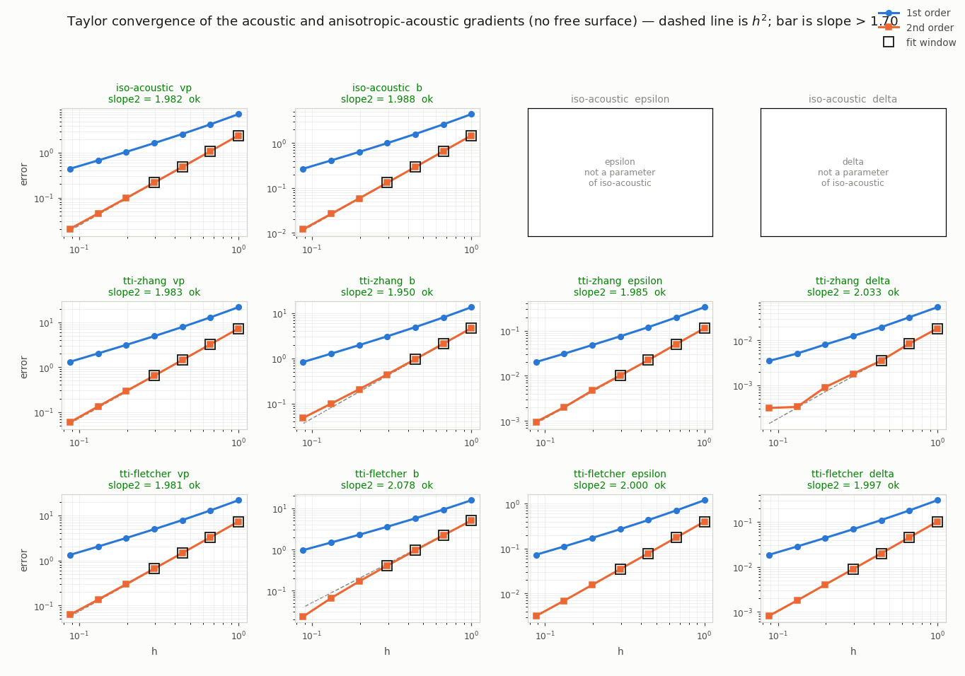
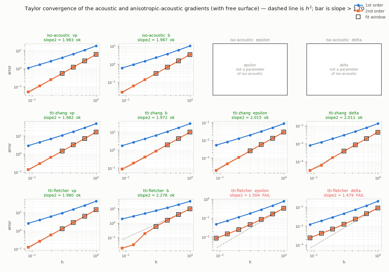
so the second-order error falls with a fitted log-log slope of 2. The assertion is one-sided (slope > 1.7): converging faster than \(h^2\) means the second-order term nearly vanishes for that perturbation, which is not an error, so an upper bound would fail correct gradients.
The adjoint dot product checks the propagator on its own, independently of any sensitivity: \(\langle Fs, r\rangle = \langle s, F^{\!\top} r\rangle\). A recipe whose adjoint is only the forward stencils run backward in time — a pseudo-adjoint — fails this even when its gradients look plausible, and the Taylor slopes alone cannot tell the two apart. It is the test to fix first when both are failing: no sensitivity can recover from an adjoint that is not the transpose.
The transpose test checks one kernel against one operator, with no wave equation and no adjoint in between: it takes the operator the propagation applies, differentiates it numerically with respect to the parameter at a few points, and compares. It is the instrument that separates a transposition mistake from a wavefield one, and it is sharp where the other two are not — a kernel can be well over a hundred per cent out pointwise here while its Taylor slope passes.
Regenerate every figure on this page with
python scripts/plot_gradients.pywhich runs the same checks as tests/test_gradient.py on a reduced model (N=101, nt=1000) that reproduces every slope to about 0.03.
1. Adjoint dot product
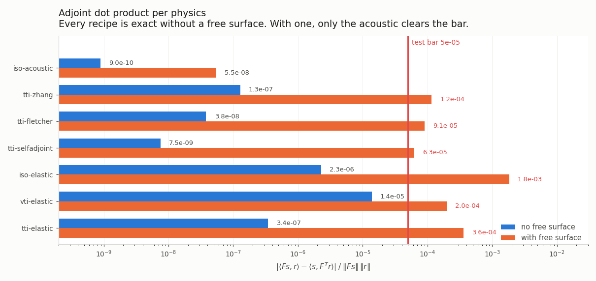
The mismatch is measured against \(\|Fs\|\,\|r\|\), the scale of the bilinear form, rather than against \(\langle Fs, r\rangle\) itself. With a random \(r\) that inner product is a largely cancelling sum whose value swings by an order of magnitude with the number of time steps, so dividing by it reports the conditioning of one draw rather than the accuracy of the transpose: the same exact adjoint reads 1.9e-5, 1.2e-4 and 1.1e-5 at 200, 400 and 800 steps.
Every recipe is exact without a free surface bar the rotated elastic one, and with one the acoustic and the elastic recipes clear the bar where the anisotropic-acoustic ones do not — see the change of variables for both, and Known limitations.
2. Acoustic and anisotropic-acoustic
3. Imaging-condition parameters
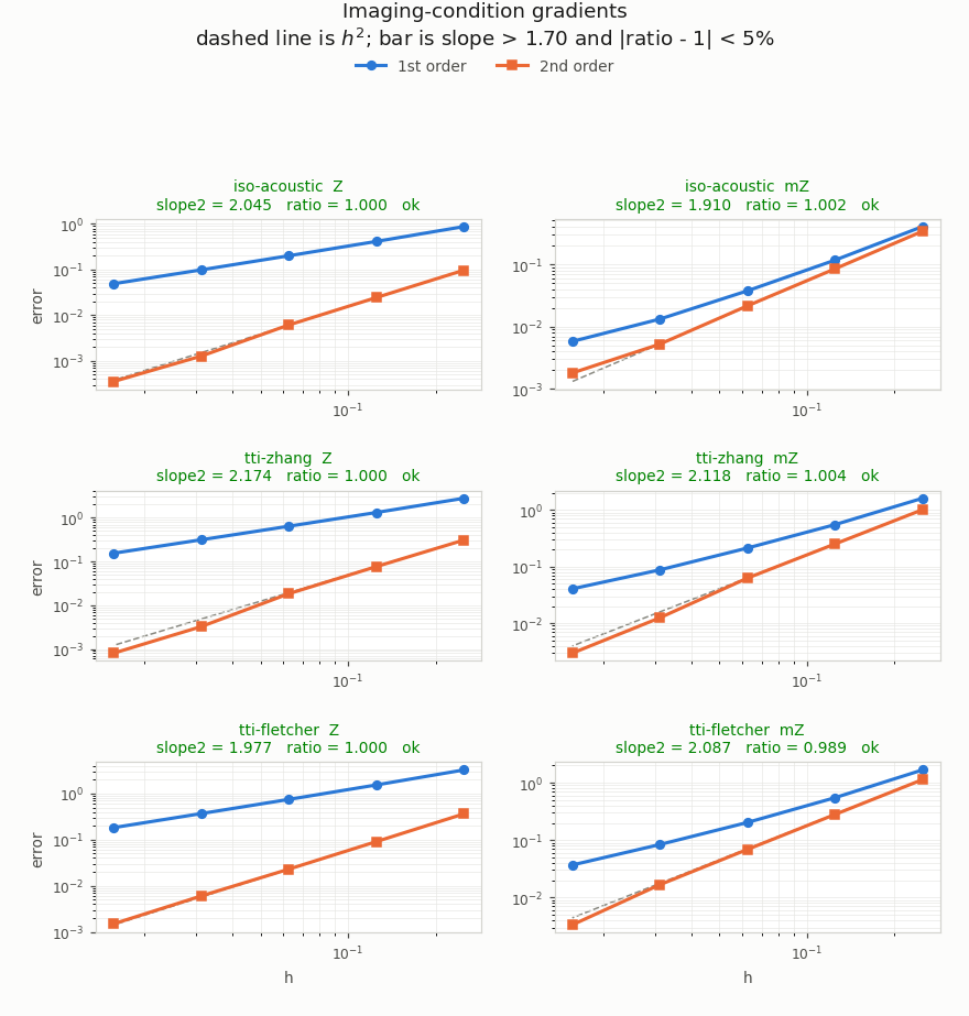
Z and mZ are the reflection-FWI pair, and neither is a stored field, so neither is perturbed directly. \(Z = \rho c\) at fixed m is a pure density move, which is why its direction is b. mZ is squared slowness at fixed impedance, so it moves both fields at once – \(\delta\ln c = -\tfrac12\delta\ln m\) and \(\delta\ln\rho = +\tfrac12\delta\ln m\) leave \(Z\) alone.
Both are built from the same two correlations the buoyancy gradient is built from, a mass one \(K_m\) and a stiffness one \(K_s\):
\[ g_m = -\mathrm{d}t\, b\, K_m, \quad g_b = -\mathrm{d}t\,(m K_m + K_s), \quad g_{mZ} = -\mathrm{d}t\,(m K_m - K_s), \]
so Z is the buoyancy gradient and mZ is \(2(m/b)g_m - g_b\) pointwise. That identity is the sharpest check available on the condition, and test_isic_slowness_composition holds it to 1e-6 – worth having, because mZ differences two kernels that can cancel to one part in 16, which amplifies a finite difference’s own error by the same factor.
Two instruments are asserted, not one, because neither subsumes the other. The panels above show the Taylor errors; the ratio \(\mathrm{d}\Phi/\mathrm{d}h \,/\, \langle g,\delta m\rangle\) by central difference is printed alongside. For Z the slope is the sharper of the two. For mZ it is not: mZ is a transmission parameter, weakly seen by a surface acquisition, so \(h\langle g,\delta m\rangle\) stays small against the curvature and the slope can rank a wrong gradient above the right one. The ratio separates them.
The fit window matters as much as the bar: \(h\in[0.015,\,0.25]\). Above it the quadratic term dominates \(\Phi(h)-\Phi(0)\) and below it error2 is at the float32 floor of a misfit summed over the whole record, and a fit spanning either reports neither.
Both sweeps run on a smooth background. m on Fletcher is the pseudo-adjoint’s gradient rather than the strict Fréchet derivative, which its own docstring says, so a background that oscillates cell to cell measures the difference between the two rather than the imaging condition.
Born
Both are linearized too, on all three recipes. The Born sources are transposed from the accumulators rather than derived again – the identities above pin them:
\[ J_Z = J_b, \qquad J_{mZ}\,q = J_m\!\left(2\tfrac{m}{b}q\right) - J_b(q), \]
and since \(J_m(x) = x\,L(u)/m\) the second collapses to the same two terms as the first with the stiffness one added instead of subtracted. Against the adjoint, \(\langle J q, d\rangle / \langle q, J^{\!\top} d\rangle\) reads 1.000005 (Z) and 1.000028 (mZ); as a Fréchet derivative the second-order error falls at 4.075 and 3.824.
mZ needs a larger perturbation than the other parameters, since its two legs cancel to about a half and the linearized signal sits closer to the float32 floor of differencing two forwards. What bounds it from above is not the amplitude of q but the exponent h*q/b, since mZ scales the velocity by exp(-h*q/b): scaled like Z that reaches 1.36, a factor 3.9 on the velocity, which the acoustic forward absorbs and Fletcher’s does not. The sweep bounds it at 0.4 instead and reads the best ratio rather than the mean, test_jacobian_forward’s convention and for its reason.
On the anisotropic recipes
The same two identities, with the stiffness written per physics. Both TTI recipes carry the buoyancy inside their stiffness operators – Gxx/Gzz for Zhang, the rotated H1/H2 for Fletcher – so the mass term is only half of d/db. Writing \(H^{(q)}\) for the stiffness evaluated with q in place of b, which is its derivative in that direction since every one of them is linear in the buoyancy,
\[ J_b\,q = (q/b)\,H - H^{(q)}, \]
the first term being Zhang’s mass term rewritten with the PDE identity and Fletcher’s vp**2/b prefactors, which its stencil carries instead of a mass term. q is passed to the operators as their b argument – they take one, and each is linear in it – rather than substituted afterwards, which would match nothing: the buoyancy enters those stencils already sampled at the half cells.
Measured: as Fréchet derivatives, b converges at 4.10 (Zhang) and 4.22 (Fletcher), Z at 4.10 to 4.22 and mZ at 3.46 to 3.91 across the three recipes. Against the adjoint, \(\langle Jq, d\rangle/\langle q,
J^{\!\top}d\rangle\) currently reads 0.930 to 0.938 for every recipe and every parameter, vp included; see Known limitations.
This check also has to run on a smooth background, and for the same reason: an inner product that cancels, taken against a pseudo-adjoint gradient, can land anywhere.
Which way the scale separation goes
Z sums the mass and stiffness kernels and mZ differences them, and the two annihilate opposite scattering angles: on a homogeneous model with one source-receiver pair, where the only event is the transmitted wave, Z retains 11 per cent of the cross-correlation kernel’s energy away from the two singular points and mZ retains 80. So Z is the reflectivity condition and mZ the transmission one, which is what the parameterization says they are and what JUDI’s ic="isic" / ic="fwi" pair does with the same signs. examples/imaging_conditions.ipynb has the picture.
4. Elastic
The change of variables
The elastic velocity–stress system is not self-adjoint as it stands. The forward is
\[ \partial_t v = b\,\nabla\!\cdot\tau, \qquad \partial_t \tau = C : \varepsilon(v), \]
and its adjoint carries \(-\partial_t\tilde\tau = \varepsilon(\tilde v)\), which is a different system. Substituting \(\sigma = C:\tilde\tau\) (Yang et al.) turns it back into the forward one, so the backward run is the forward stencils stepped backward in time – free surface, water layer and fluid mask included – and the change of variables is undone in the three places that read \(\sigma\):
| forward | backward | |
|---|---|---|
| stress source | inject into \(\tau_{ii}\) | inject \(C:I\) |
| recorded field | \(\mathrm{tr}(\tau)\) | \(\mathrm{tr}(C^{-1}\sigma)\) |
| stiffness sensitivity | – | \(\tilde\tau_a\,\hat e_b(v)\) with \(\tilde\tau = C^{-1}\sigma\) |
\(C^{-1}\) is closed form for an isotropic \(C\), and is written as its isotropic plus deviatoric halves rather than as \((t - \lambda\,\mathrm{tr}(t)/lm)/2\mu\): the two are the same expression rearranged, but split that way the guard on \(1/2\mu\) takes the deviatoric half alone and a fluid keeps \(\mathrm{tr}(C^{-1}t) = \mathrm{tr}(t)/n\lambda\) – which is what the adjoint measurement of a marine acquisition reads. For an anisotropic \(C\) the inverse is taken in the crystal frame, where the VTI matrix is a normal block plus a diagonal shear block, and the rotation is undone on the tensor rather than on the matrix: a rotation is orthogonal on the space of symmetric tensors, so rotating the inverse and inverting the rotated \(6\times6\) are the same thing, and only one of the two needs a symbolic inverse. A fluid falls back on the isotropic form, which is exact there rather than approximate – \(\epsilon\) and \(\delta\) vanish with \(v_s\). test_elastic_compliance_inverts_stiffness measures the round trip at 1e-7 in float32, 3D TTI included, and test_elastic_compliance_fluid_trace the fluid limit.
What it buys is the free surface. A self-adjoint operator run backward is its own transpose, mirror and all, which is what makes iso-acoustic pass the dot product at fs=True. Measured on the propagator, 400 steps, before and after the change of variables:
| recipe | fs=False |
fs=True |
|---|---|---|
iso-elastic |
2.3e-6 -> 2.7e-7 | 4.5e-3 -> 3.9e-8 |
vti-elastic |
1.4e-5 -> 4.6e-8 | 1.7e-3 -> 8.4e-5 |
tti-elastic |
3.4e-7 -> 1.3e-4 | 3.1e-3 -> 1.7e-3 |
What it costs is the rotated stiffness without a free surface. On a staggered grid a rotated \(C\) couples the normal stress components, which sit on the node, to the shear ones, which sit on the cell corners, so the discrete change of variables carries an interpolation between the two and is no longer pointwise. It does not appear on vti-elastic, whose stiffness couples only components that share a location, nor on iso-elastic, and it is the same cross-staggering that tti-elastic’s epsilon/delta gradients trip over. test_adjoint_dot_product carries the 1.3e-4 as a documented per-recipe tolerance rather than a blanket one.
The coefficients have to be Devito expressions
A rotated stiffness is the case where the placement of a staggered product decides whether the discrete \(\mathbf{C}\) is its own transpose, and the staggered-interpolation tutorial is the reference: interpolating each factor to the target gives \(\langle C\rangle\langle\varepsilon\rangle\) where the transpose needs \(\langle C\varepsilon\rangle\). Measured on this stiffness, on a model rough enough for the two to differ, \(\langle Cx, y\rangle\) against \(\langle x, Cy\rangle\) reads
direct |
symmetric |
|
|---|---|---|
tti-elastic |
4.3e-2 | 4.5e-7 |
vti-elastic |
8.7e-8 | 8.7e-8 |
iso-elastic |
5.7e-8 | 5.7e-8 |
For those placement decisions to apply at all, the coefficients have to reach Devito as Differentiable expressions. SeismicStiffness builds them against sympy placeholders – the 3⁸ rotation loop is far cheaper that way – so they are substituted back with devito_subs, which goes through Devito’s own operators; a plain xreplace rebuilds the tree with sympy’s Add and Mul, and the Functions inside become invisible to the interpolation machinery.
The propagation itself uses direct rather than symmetric. sensitivity_eqs accumulates the derivative of the stress update as direct places it, and the two have to agree; switching the propagation is a re-derivation of the kernel rather than a flag, and it does not close the tti-elastic dot product either. The measurements behind that choice are in docs/elastic_gradients_status.md.
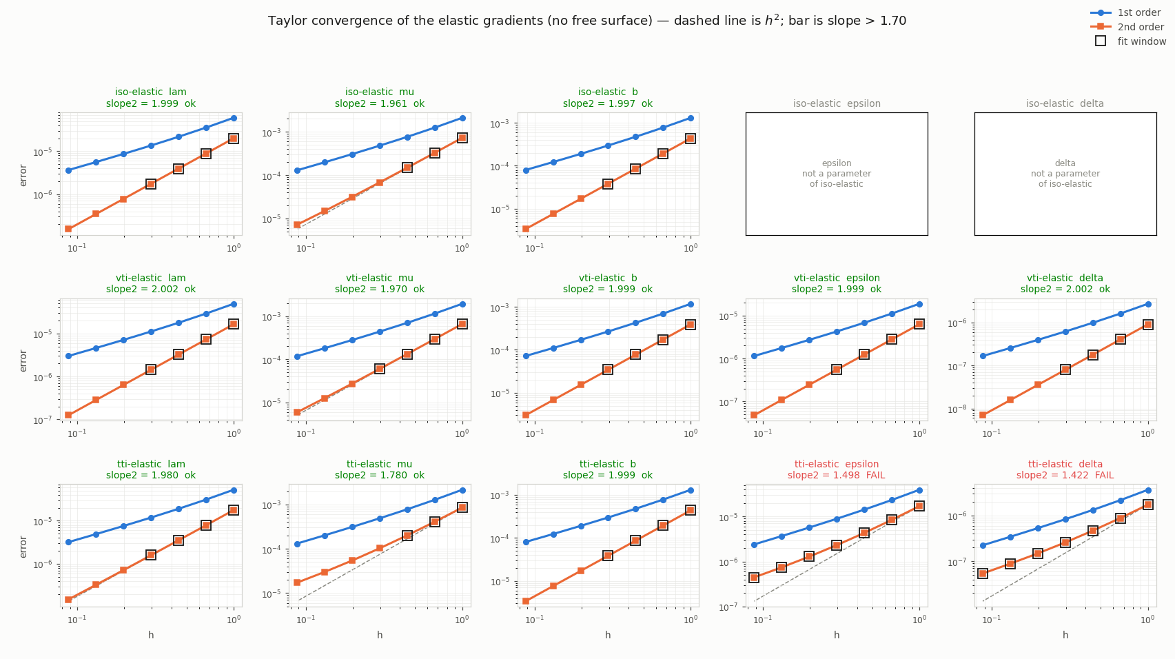
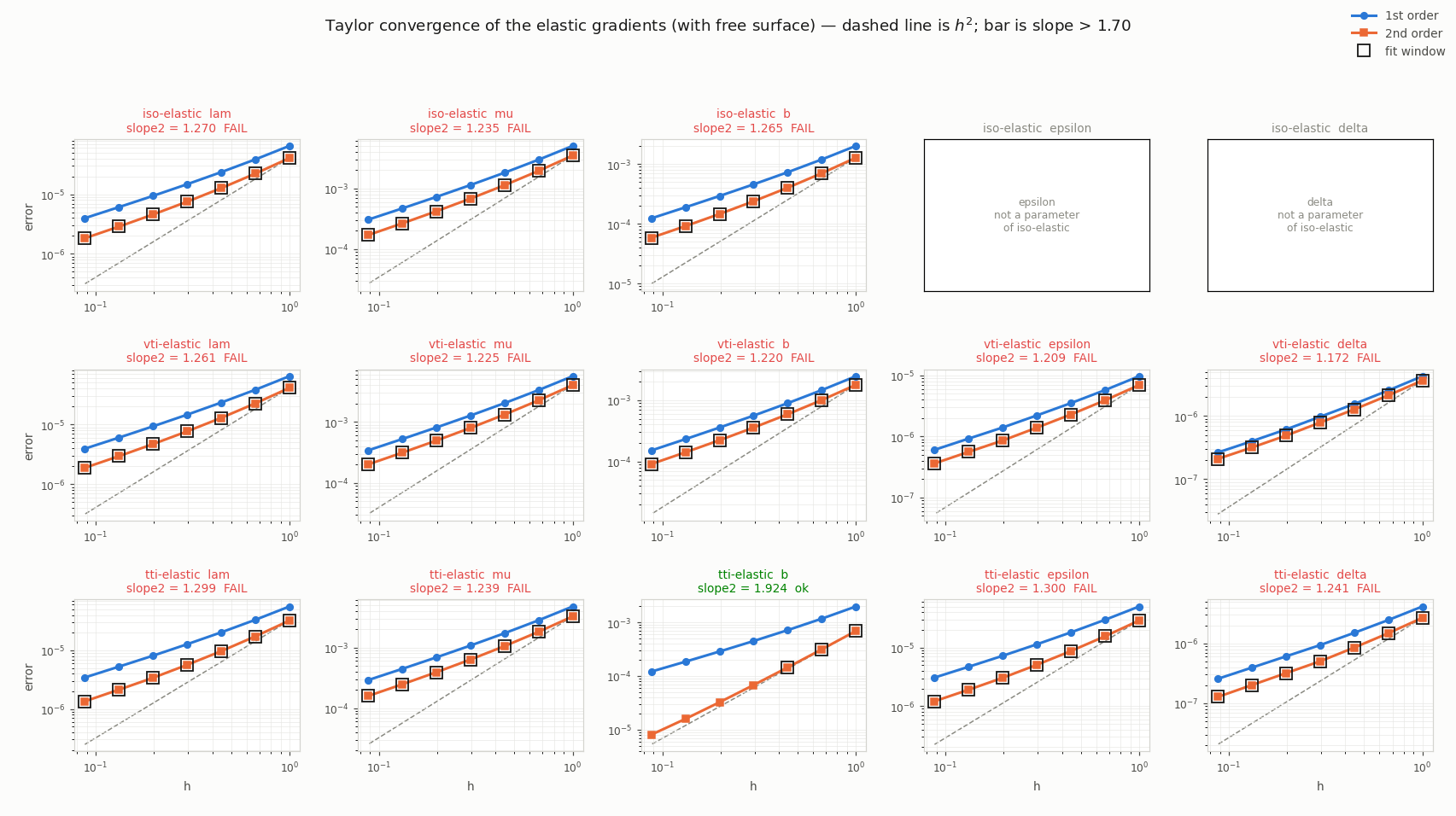
vp and vs do not appear: an elastic model stores the Lamé parameters, the stiffness is assembled from them, and the propagation never reads a velocity, so perturbing model.vp leaves it untouched and there is nothing to Taylor test against. They reach the stiffness through \(\lambda = v_p^2/\rho - 2v_s^2\) and \(\mu = v_s^2/\rho\), and test_elastic_velocity_chain_rule checks them against the lam/mu gradients, which are tested here.
5. Known limitations
| Case | Symptom |
|---|---|
| Accumulated gradient magnitude | about 7 per cent high across recipes and parameters: the imaging-condition ratios read 0.925 to 0.936 against a 5 per cent bar, and the Born/adjoint pair reads 0.930 to 0.938 for every recipe and parameter, vp included. The kernels themselves each pass the transpose test, and the Born sources converge at 4 |
The anisotropic-acoustic recipes, fs=True |
the propagator is not the transpose — 6e-5 (tti-selfadjoint) upwards. The elastic ones are no longer here: the change of variables makes them self-adjoint, and iso-elastic reads 3.9e-8 |
iso-elastic and tti-elastic mu, fs=True, and tti-elastic b there |
what is left of the above — every other elastic gradient converges, lam and the Thomsen parameters included. b fails only where the stiffness is rotated (1.46), and only with a free surface |
tti-elastic, fs=False, dot product |
1.3e-4 against 5e-5 — a rotated stiffness couples components that live on different staggered positions, so the change of variables is not pointwise |
tti-fletcher epsilon/delta, fs=True |
slope 1.50 / 1.48 |
tti-fletcher b/Z images |
grid-scale ringing from the expanded operator form — the gradient is exact (0.9995), the image is not smooth |
Z/mZ Born on the TTI recipes |
tti-fletcher has no b Born source and tti-zhang’s carries only the mass term |
These are xfailed in tests/test_gradient.py rather than silently loosened; the bar stays at 2 for everything else.