Expanding box

In seismic modeling and inversion, and more generally when simulating the solution of hyperbolic equations, it is well known that the wavefront will progressively fill the entire computational domain starting from the source position. This means that the computational domain should be reduced to the imprint of the wavefield to improve performance. Such a construct is called an expanding box, and is implemented with ABox in devitopro.

In this notebook, we show how to use ABox to improve the performance of the discrete propagators for the forward modeling, adjoint modeling, and the computation of the gradient (combination of the forward and adjoint modeling)

The core idea behind the implementation of an expanding box is that, given a spatial and temporal discretization \(h_x, h_y,h_z, dt\) then we know that at a given timestep, enforced by the CFL condition, the wavefield can progress at most by a distance

\[ d_\text{expand}(x, y, z) = v(x, y, z) dt \]

which means, for a rectangular box, we need to extend the domain at each time step by

\[\begin{equation} \begin{aligned} e_{xl} &= \text{max}(v(x_{bl}, y, z)) dt \\ e_{xr} &= \text{max}(v(x_{br}, y_{br}, z)) dt \\ e_{yl} &= \text{max}(v(x, y_{bl}, z)) dt \\ e_{yr} &= \text{max}(v(x, y_{br}, z)) dt \\ e_{zl} &= \text{max}(v(x, y, z_{bl})) dt \\ e_{zr} &= \text{max}(v(x, y, z_{br})) dt \\ \end{aligned} \end{equation}\]

where \(x_{bl/r}, y_{bl/r}, z_{bl/r}\) are the current left/right limits of the computational domain. In DevitoPRO, we precompute those limits at each timestep based on the source position, discretization, and velocity.

Anisotropic velocity

In the case of anisotropy, i.e in a VTI or TTI medium, the velocity along the fast axis is increased by a factor \(\sqrt{1 + 2 \epsilon}\), where \(\epsilon\) is the Thomsen parameter. This means that the expanding box should be increased by the same factor. In DevitoPRO, we precompute the expanding box for the fast axis and then multiply the expanding box by \(\sqrt{1 + 2 \epsilon}\) to get the expanding box for the slow axis. In practice, the expanding box method is called with the extra eps parameter:

abox = ABox(src, rec, vp, sradius, eps=epsilon)

For illustrative purposes, we set up this example in an acoustic isotropic medium. Usage of ABox in a TTI medium can be found in the demos:

from devitopro import *
from devito import TimeFunction, Eq, Operator, solve, configuration
configuration["log-level"]="ERROR"

from IPython.display import HTML
import matplotlib.pyplot as plt
import matplotlib.animation as animation

def make_animation(u, model, abox=None, rev=False, snapshotregion=None):
    nx, ny = model.grid.shape

    if snapshotregion is None:
        extent = (0, nx, ny, 0)
    else:
        extent = (snapshotregion[0], nx-snapshotregion[1], ny-snapshotregion[2], snapshotregion[3])

    t0 = (u.shape[0]-1) if rev else 0
    cv = 50 if rev else 1

    fig, ax = plt.subplots()
    im = ax.imshow(u.data[t0, :, :].T, vmin=-cv, vmax=cv, cmap="seismic", extent=extent)
    im2 = ax.imshow(model.vp.data.T, vmin=1.5, vmax=3.5, cmap="jet", alpha=.5, extent=(0, nx, ny, 0))

    if abox is not None:
        abox = abox._compute(dt=model.critical_dt, nt=u.shape[0])
        x = [abox[t0, 0], nx-abox[t0, 1], nx-abox[t0, 1], abox[t0, 0], abox[t0, 0]]
        y = [abox[t0, 2], abox[t0, 2], ny-abox[t0, 3], ny-abox[t0, 3], abox[t0, 2]]

        line, = plt.plot(x, y, c='orange', linewidth=3.0)
    else:
        line = None

    if snapshotregion is not None:
        x = [snapshotregion[0], nx-snapshotregion[1], nx-snapshotregion[1], snapshotregion[0], snapshotregion[0]]
        y = [snapshotregion[3], snapshotregion[3], ny-snapshotregion[2], ny-snapshotregion[2], snapshotregion[3]]
        plt.plot(x, y, 'k--', linewidth=3.0)

        if abox is not None:
            x = [max(abox[t0, 0], snapshotregion[0]), nx-max(abox[t0, 1], snapshotregion[1]),
                 nx-max(abox[t0, 1], snapshotregion[1]), max(abox[t0, 0], snapshotregion[0]),
                 max(abox[t0, 0], snapshotregion[0])]

            y = [max(abox[t0, 2], snapshotregion[3]), max(abox[t0, 2], snapshotregion[3]),
                 ny-max(abox[t0, 3], snapshotregion[2]), ny-max(abox[t0, 3], snapshotregion[2]),
                 max(abox[t0, 2], snapshotregion[3])]
            line2, = plt.plot(x, y, 'r', linewidth=3.0)
        else:
            line2 = None
    else:
        line2 = None
            

    plt.xlabel('x')
    plt.ylabel('z')
    ax.set_title("{time:.2f}sec".format(time=1e-3*t0*model.critical_dt))

    def update(i, im, line):
        time = (u.shape[0] - i*10 - 1) if rev else i*10
        im.set_array(u.data[time, :, :].T)
        ax.set_title("{time:.2f}sec".format(time=1e-3*time*model.critical_dt))

        artists = [im]

        if abox is not None:
            x = [abox[time, 0], nx-abox[time, 1], nx-abox[time, 1], abox[time, 0], abox[time, 0]]
            y = [abox[time, 2], abox[time, 2], ny-abox[time, 3], ny-abox[time, 3], abox[time, 2]]
            line.set_data(x, y)
            artists.append(line)

            if snapshotregion is not None:
                x = [max(abox[time, 0], snapshotregion[0]), nx-max(abox[time, 1], snapshotregion[1]),
                     nx-max(abox[time, 1], snapshotregion[1]), max(abox[time, 0], snapshotregion[0]),
                     max(abox[time, 0], snapshotregion[0])]
                y = [max(abox[time, 2], snapshotregion[3]), max(abox[time, 2], snapshotregion[3]),
                     ny-max(abox[time, 3], snapshotregion[2]), ny-max(abox[time, 3], snapshotregion[2]),
                     max(abox[time, 2], snapshotregion[3])]
                line2.set_data(x, y)
                artists.append(line2)

        return artists

    # Animation
    nsnaps = u.shape[0] // 10
    ani = animation.FuncAnimation(fig, update, fargs=[im, line], frames=nsnaps, interval=50, blit=True)

    return ani

Setup

Let’s start with setting up a simple 2D acoustic model with a single source in the middle and receivers all over the surface. This will help visualize the concept and easily show how to use the API. The current implementation supports acoustic and anisotropic wave equations.

from examples.seismic import demo_model, setup_geometry

so = 4
model = demo_model('layers-isotropic', shape=(201, 201), spacing=(10., 10.), space_order=so, nbl=40)
geometry = setup_geometry(model, 1250)

src, rec = geometry.src, geometry.rec
recfull, recf, recfb = geometry.rec, geometry.rec, geometry.rec

# Setup the receivers as OBN, i.e different depth than the source for illustrative purposes
rec.coordinates.data[:, -1] = 650
recfull.coordinates.data[:, -1] = 650
recf.coordinates.data[:, -1] = 650
recfb.coordinates.data[:, -1] = 650

from examples.seismic import plot_velocity

plot_velocity(model, source=src.coordinates.data,
              receiver=rec.coordinates.data)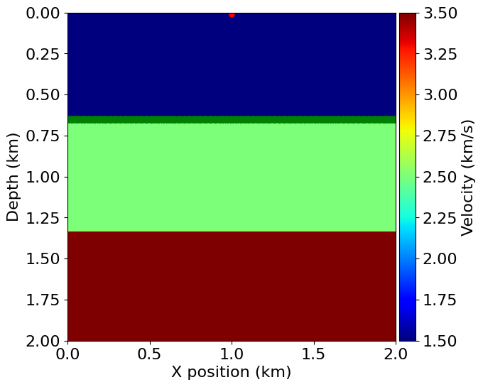

from devitopro.subdomains import ABox

# Source expanding box, for forward propagation
aboxsrc = ABox(src, None, model.vp, so, name="aboxsrc")
# Receiver expanding box, for backward propagation. If the user wish to use a forward propagation with the receivers as a source
# then ABox(rec, None, model.vp, so, name="aboxsrc") should be used
aboxrec = ABox(None, rec, model.vp, so, name="aboxrec")
# Source and receiver expanding box combining the domain of the forward abd adjoint wavefronts
aboxsrcrec = ABox(src, rec, model.vp, so, name="aboxsrcrec")

Propagation

We now create a propagator for the wave equation and visualize the effect of the expanding box

u = TimeFunction(name="u", grid=model.grid, space_order=so, time_order=2, save=src.shape[0])
ub = TimeFunction(name="u", grid=model.grid, space_order=so, time_order=2, save=src.shape[0])
ufb = TimeFunction(name="u", grid=model.grid, space_order=so, time_order=2, save=src.shape[0])
ufull = TimeFunction(name="u", grid=model.grid, space_order=so, time_order=2, save=src.shape[0])

eq = model.m * u.dt2 - u.laplace + model.damp * u.dt
eqb = model.m * u.dt2 - u.laplace + model.damp * u.dt.T

stencil = Eq(u.forward, solve(eq, u.forward), subdomain=aboxsrc)

srceq = src.inject(u.forward, expr=src)
receq = rec.interpolate(u)
recsrc = rec.inject(u.backward, expr=rec)

Source expanding box

In this first case, we consider the expanding box that follows the forward wavefield from a point source. The box starts as a small, almost empty, box around the source position with a width of the chosen spatial discretization order. The box then progressively expands until the computational domain reaches the edges.

op = Operator([stencil] + srceq + receq)
summary = op(dt=model.critical_dt, u=u, rec=recf)

# NBVAL_SKIP
ani = make_animation(u, model, abox=aboxsrc)
plt.close(ani._fig)
HTML(ani.to_html5_video())

Receiver expanding box

In this second case, we consider the receiver side box that is computed for backward propagation. This box corresponds to the “source expanding box” considering the receivers as sources and a time reverse propagation. We see that the box starts as a narrow rectangle encompassing all the ocean bottom nodes and progressively (ib backward times) fills the whole domain.

stencil = Eq(u.backward, solve(eqb, u.backward), subdomain=aboxrec)
op = Operator([stencil] + recsrc)
summary = op(dt=model.critical_dt, u=ub, rec=recf)

# NBVAL_SKIP
ani = make_animation(ub, model, abox=aboxrec, rev=True)
plt.close(ani._fig)
HTML(ani.to_html5_video())

Source and receiver expanding box

Finally we look at the composition of the forward source box and the backward receiver box. In addition for taking into account the propagation of the forward wavefield, the box is shrinking towards the end of the propagation cutting out any area containing a wavefield that cannot physically reach a receiver anymore. This leads to an expanding from the source then shrinking towards the OBNs box.

stencil = Eq(u.forward, solve(eq, u.forward), subdomain=aboxsrcrec)
op = Operator([stencil] + srceq + receq)
summary = op(dt=model.critical_dt, u=ufb, rec=recfb)

# NBVAL_SKIP
ani = make_animation(ufb, model, abox=aboxsrcrec)
plt.close(ani._fig)
HTML(ani.to_html5_video())

Shot records comparison

We finally show that using an expanding box ads to negligible effects to the recorded synthetic data. We first compute the data without an expanding box for reference.

stencil = Eq(u.forward, solve(eq, u.forward))
op = Operator([stencil] + srceq + receq)
summary = op(dt=model.critical_dt, u=ufull, rec=recfull)

extent = [recfull.coordinates.data[0, 0], recfull.coordinates.data[-1, 0], 1.25, 0]

plt.figure(figsize=(9,6))
plt.subplot(1,3,1)
plt.imshow(recfull.data, vmin=-.5, vmax=.5, cmap="seismic", extent=extent, aspect="auto")
plt.xlabel("X (m)")
plt.ylabel("Time (s)")
plt.title("No ABox")
plt.subplot(1,3,2)
plt.imshow(recf.data, vmin=-.5, vmax=.5, cmap="seismic", extent=extent, aspect="auto")
plt.xlabel("X (m)")
plt.ylabel("Time (s)")
plt.title("Source ABox")
plt.subplot(1,3,3)
plt.imshow(recfb.data, vmin=-.5, vmax=.5, cmap="seismic", extent=extent, aspect="auto")
plt.xlabel("X (m)")
plt.ylabel("Time (s)")
plt.title("SourceRec ABox")
plt.tight_layout()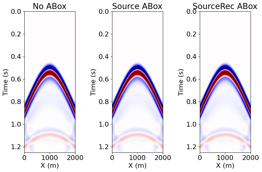

We see that the shot records match very well. We additionally show below that the difference is extremely small (near floating point precision) making the use of the expanding box suitable for modelling and inversion

plt.figure(figsize=(6,6))
plt.suptitle("Error (x1e5)")
plt.subplot(1,2,1)
plt.imshow(recf.data-recfull.data, vmin=-5e-5, vmax=5e-5, cmap="seismic", extent=extent, aspect="auto")
plt.xlabel("X (m)")
plt.ylabel("Time (s)")
plt.title("Source ABox")
plt.subplot(1,2,2)
plt.imshow(recfb.data-recfull.data, vmin=-5e-5, vmax=5e-5, cmap="seismic", extent=extent, aspect="auto")
plt.xlabel("X (m)")
plt.ylabel("Time (s)")
plt.title("SourceRec ABox")
plt.tight_layout()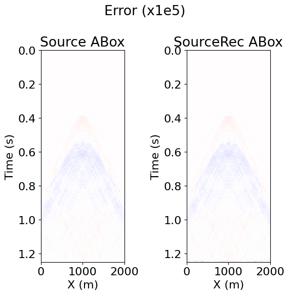

Combining `ABox` with `Function`s on `SubDomain`s

For certain applications, one may only require a field to be present on a subset of the domain. One such example is snapshotting, where the damping layers at the edge of the domain can be trimmed off, as they are not needed for imaging. The Functions on SubDomains API is used to achieve this, and can be straightforwardly combined with ABox.

First, we create a SubDomain that excludes the damping layers.

from devito import SubDomain

class SnapshotDomain(SubDomain):
    """Snapshot region trimming off the boundary layers"""
    name = 'snapshot'

    def __init__(self, nbl=0, grid=None):
        self.nbl = nbl
        super().__init__(grid=grid)

    def define(self, dimensions):
        return {d: ('middle', self.nbl, self.nbl) for d in dimensions}


snapshotdomain = SnapshotDomain(nbl=40, grid=model.grid)

We then create our snapshot TimeFunction. Note that one would usually use a ConditionalDimension for time, but this is omitted for simplicity. This TimeFunction is defined only on the snapshotdomain.

usave = TimeFunction(name="usave", grid=snapshotdomain, space_order=so, time_order=2, save=src.shape[0])

For the iteration, it is necessary to intersect the snapshotdomain with our ABox, in this case aboxsrcrec. This is to keep iteration within the snapshotdomain. Using the ABox includes points outside the snapshotdomain, resulting in out-of-bounds memory accesses when operating on usave.

snapshotbox = aboxsrcrec.intersection(snapshotdomain, name='snapshotbox')

We can then create our Eq, passing in the snapshotbox.

# `ufull` is already populated, so no need to update it
snap_eq = Eq(usave, ufull, subdomain=snapshotbox)
op = Operator(snap_eq)

And run the Operator…

summary = op(dt=model.critical_dt)

Finally, plotting the snapshotted wavefield, we see that it is present on a reduced area of the domain. We also see the intersected ABox plotted in red.

# NBVAL_SKIP
ani = make_animation(usave, model, abox=aboxsrcrec, snapshotregion=(40, 40, 40, 40))
plt.close(ani._fig)
HTML(ani.to_html5_video())