from recipes import layered_model, recipes_registry
import matplotlib.pyplot as pltElastic FWI
This notebook provide a brief overview of the interface for elastic inversion, in particular which gradients are available and how to compute them. We currently only support isotropic elastic mode. While we do provide a TTI elastic solver, the TTI kernel are only implementing the forward modeling and not the sensitivities at the moment.
Free surface
Additionally, the elastic solver supports acoustic free surface for marine case where the surface is known to be acoustic. The operator setup will check that the S-wave velocity vs is zero at the surface.
Acquisition
Currently, the elastic solvers are setup for pressure, meaning the source is injected into the diagonal of the stress (\(\tau_{xx}, \tau_{yy}, \tau_{zz}\)) and the receiver are measuring the trace of the strain (\(\tau_{xx} + \tau_{yy} + \tau_{zz}\)).
For the purpose of didactic clarity, we will consider a simple 2D elastic model, with a single source and a line of receiver.
so = 8
nt = 2000
dt = .75
model = layered_model('iso-elastic', nlayers=4, shape=(301, 151), spacing=(10., 10.),
density=True, nbl=40, space_order=so, fs=True, dt=dt)
extent = (model.grid.origin[0], model.grid.origin[0]+model.grid.extent[0],
model.grid.origin[1]+model.grid.extent[1], model.grid.origin[1])
model.physical_params(){'vp': vp(x, y), 'lam': lam(x, y), 'mu': mu(x, y), 'b': b(x, y)}plt.figure(figsize=(12, 6))
plt.subplot(221)
plt.imshow(model.vp.data.T, cmap="jet", aspect="auto", extent=extent)
plt.colorbar()
plt.title("P-wave velocity")
plt.xlabel("x [m]")
plt.ylabel("Depth [m]")
plt.subplot(222)
plt.imshow(model.b.data.T, cmap="jet", aspect="auto", extent=extent)
plt.colorbar()
plt.title("Buoyancy")
plt.xlabel("x [m]")
plt.ylabel("Depth [m]")
plt.subplot(223)
plt.imshow(model.mu.data.T, cmap="jet", aspect="auto", extent=extent)
plt.colorbar()
plt.title(r"S-wave velocity (Lame parameter \mu")
plt.xlabel("x [m]")
plt.ylabel("Depth [m]")
plt.tight_layout()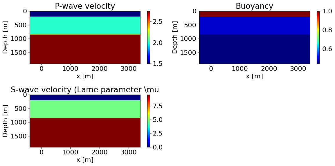
solver = recipes_registry['iso-elastic'](model, {'nt': nt, 'space_order': so, 't_sub': 8, 'f0': 0.015, 'save': None, 'time_slots': 1})Note: At the moment we recommend using either disk or None (in RAM) for saving as the other modes are untested for elastic
True data
solver.forward()Operator `initdamp` ran in 0.01 s
Operator `ForwardElasticIsotropic` ran in 0.54 sPerformanceSummary([(PerfKey(name='section0', rank=None),
PerfEntry(time=0.46358200000000066, gflopss=0.0, gpointss=0.0, oi=0.0, ops=0, itershapes=[])),
(PerfKey(name='section1', rank=None),
PerfEntry(time=0.020268999999999978, gflopss=0.0, gpointss=0.0, oi=0.0, ops=0, itershapes=[])),
(PerfKey(name='section2', rank=None),
PerfEntry(time=0.026324999999999932, gflopss=0.0, gpointss=0.0, oi=0.0, ops=0, itershapes=[])),
(PerfKey(name='section3', rank=None),
PerfEntry(time=0.021561000000000042, gflopss=0.0, gpointss=0.0, oi=0.0, ops=0, itershapes=[]))])true_data = solver.rec.data.copy()
plt.figure(figsize=(12, 6))
plt.imshow(true_data, cmap='seismic', aspect='auto', vmin=-1e-1, vmax=1e-1, extent=(0, 3000, 1.75, 0))
plt.xlabel('Receiver positon [m]')
plt.ylabel('Time [s]')Text(0, 0.5, 'Time [s]')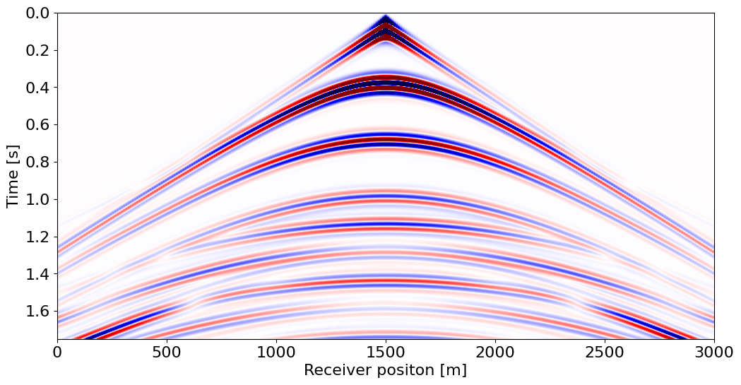
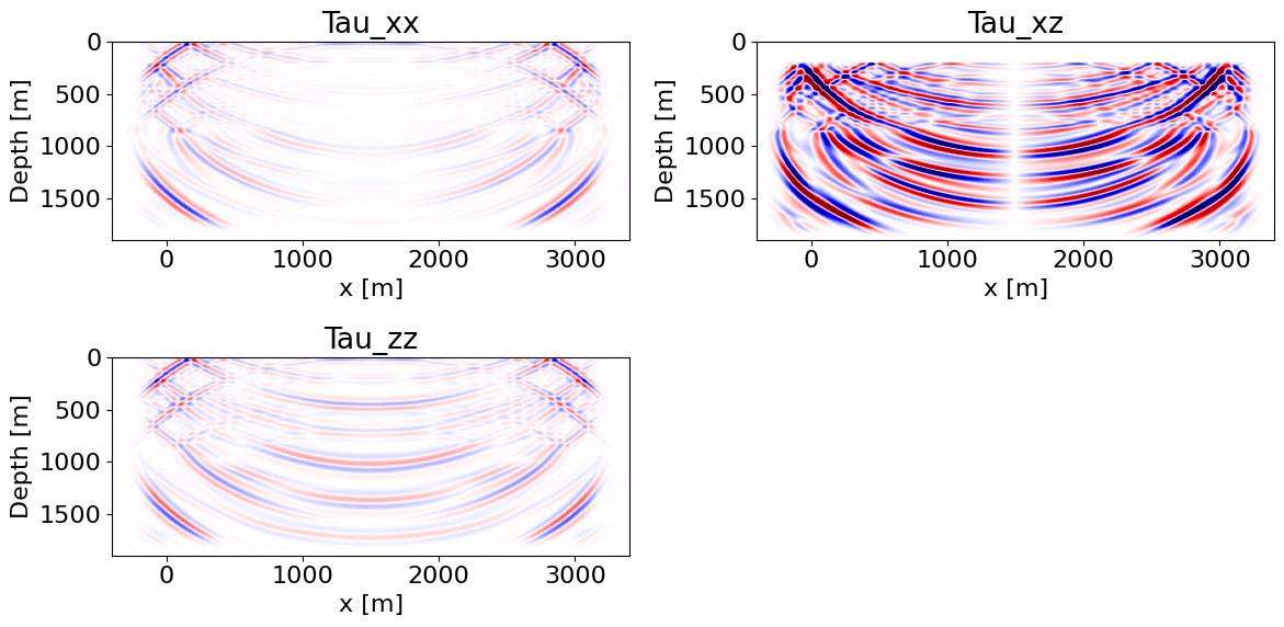
Wavefield
Let’s briefly look at the wavefield snapshots
tau, v = solver.state['tau'], solver.state['v']

plt.figure(figsize=(12, 3))
plt.subplot(121)
plt.imshow(v[0].data[0].T, cmap="seismic", aspect="auto", extent=extent, vmin=-1e-1, vmax=1e-1)
plt.title("Vx")
plt.xlabel("x [m]")
plt.ylabel("Depth [m]")
plt.subplot(122)
plt.imshow(v[1].data[0].T, cmap="seismic", aspect="auto", extent=extent, vmin=-1e-1, vmax=1e-1)
plt.title("Vz")
plt.xlabel("x [m]")
plt.ylabel("Depth [m]")
plt.tight_layout()

plt.figure(figsize=(12, 6))
plt.subplot(221)
plt.imshow(tau[0].data[0].T, cmap="seismic", aspect="auto", extent=extent, vmin=-1e-1, vmax=1e-1)
plt.title("Tau_xx")
plt.xlabel("x [m]")
plt.ylabel("Depth [m]")
plt.subplot(222)
plt.imshow(tau[1].data[0].T, cmap="seismic", aspect="auto", extent=extent, vmin=-1e-2, vmax=1e-2)
plt.title("Tau_xz")
plt.xlabel("x [m]")
plt.ylabel("Depth [m]")
plt.subplot(223)
plt.imshow(tau[3].data[0].T, cmap="seismic", aspect="auto", extent=extent, vmin=-1e-1, vmax=1e-1)
plt.title("Tau_zz")
plt.xlabel("x [m]")
plt.ylabel("Depth [m]")
plt.tight_layout()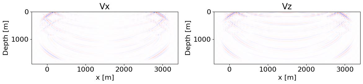
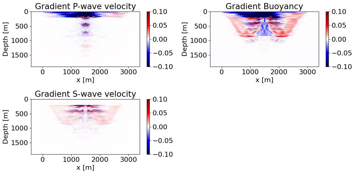
Gradients
Let’s now compute the gradients. For elastic isotropic, there is three independent parameters: \(\rho\), \(vp\) and \(vs\). THose three gradients are accessible through the params argument of the jacobian_adjoint methods.
We will compute a simple gradient in a smooth model by first computing the background data in the smooth model then computing all three gradients.
model0 = layered_model('iso-elastic', nlayers=4, shape=(301, 151), spacing=(10., 10.),
                      density=True, nbl=40, space_order=so, fs=True, dt=dt)
model0.smooth(['vp', 'lam', 'mu', 'b'])
solver.forward(vp=model0.vp, vs=model0.vs, b=model0.b, save=True)
Operator `ForwardElasticIsotropic` ran in 0.55 sPerformanceSummary([(PerfKey(name='section0', rank=None),
PerfEntry(time=0.46136399999999944, gflopss=0.0, gpointss=0.0, oi=0.0, ops=0, itershapes=[])),
(PerfKey(name='section1', rank=None),
PerfEntry(time=0.01976299999999996, gflopss=0.0, gpointss=0.0, oi=0.0, ops=0, itershapes=[])),
(PerfKey(name='section2', rank=None),
PerfEntry(time=0.02607499999999992, gflopss=0.0, gpointss=0.0, oi=0.0, ops=0, itershapes=[])),
(PerfKey(name='section3', rank=None),
PerfEntry(time=0.012071999999999992, gflopss=0.0, gpointss=0.0, oi=0.0, ops=0, itershapes=[])),
(PerfKey(name='section4', rank=None),
PerfEntry(time=0.02149400000000004, gflopss=0.0, gpointss=0.0, oi=0.0, ops=0, itershapes=[]))])plt.figure(figsize=(12, 6))
plt.subplot(131)
plt.imshow(true_data, cmap='seismic', aspect='auto', vmin=-1e-1, vmax=1e-1, extent=(0, 3000, 1.75, 0))
plt.xlabel('Receiver positon [m]')
plt.ylabel('Time [s]')
plt.title('True data')
plt.subplot(132)
plt.imshow(solver.rec.data, cmap='seismic', aspect='auto', vmin=-1e-1, vmax=1e-1, extent=(0, 3000, 1.75, 0))
plt.xlabel('Receiver positon [m]')
plt.ylabel('Time [s]')
plt.title('Backround data')
plt.subplot(133)
plt.imshow(solver.rec.data - true_data, cmap='seismic', aspect='auto', vmin=-1e-1, vmax=1e-1, extent=(0, 3000, 1.75, 0))
plt.xlabel('Receiver positon [m]')
plt.ylabel('Time [s]')
plt.title('Residual')
plt.tight_layout()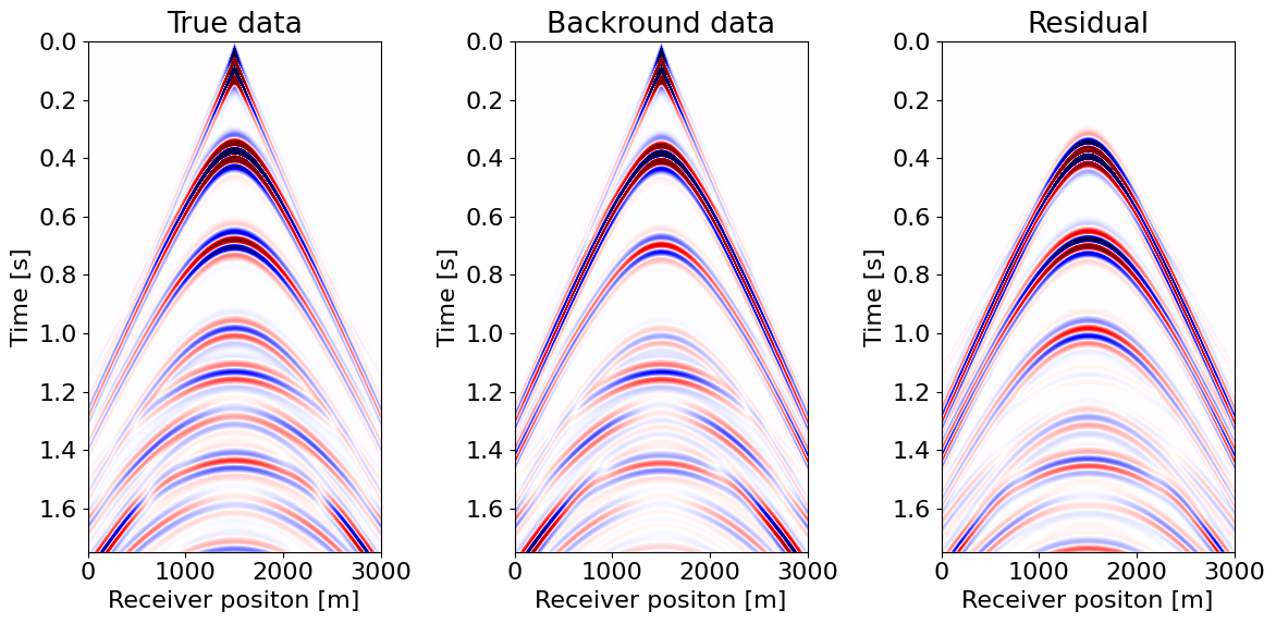
residual = solver.rec.copy()
residual.data[:] -= true_data
solver.jacobian_adjoint(params=('vp', 'vs', 'b'), vp=model0.vp, vs=model0.vs, b=model0.b, rec=residual)
Operator `JacobianAdjElasticIsotropic` ran in 0.60 sPerformanceSummary([(PerfKey(name='section0', rank=None),
PerfEntry(time=0.46099700000000066, gflopss=0.0, gpointss=0.0, oi=0.0, ops=0, itershapes=[])),
(PerfKey(name='section1', rank=None),
PerfEntry(time=0.05042899999999996, gflopss=0.0, gpointss=0.0, oi=0.0, ops=0, itershapes=[])),
(PerfKey(name='section2', rank=None),
PerfEntry(time=0.025322000000000004, gflopss=0.0, gpointss=0.0, oi=0.0, ops=0, itershapes=[])),
(PerfKey(name='section3', rank=None),
PerfEntry(time=0.05441199999999999, gflopss=0.0, gpointss=0.0, oi=0.0, ops=0, itershapes=[]))])plt.figure(figsize=(12, 6))
plt.subplot(221)
plt.imshow(solver.perturbation(param='vp').data.T, cmap="seismic", aspect="auto", extent=extent, vmin=-1e-1, vmax=1e-1)
plt.colorbar()
plt.title("Gradient P-wave velocity")
plt.xlabel("x [m]")
plt.ylabel("Depth [m]")
plt.subplot(222)
plt.imshow(solver.perturbation(param='b').data.T, cmap="seismic", aspect="auto", extent=extent, vmin=-1e-1, vmax=1e-1)
plt.colorbar()
plt.title("Gradient Buoyancy")
plt.xlabel("x [m]")
plt.ylabel("Depth [m]")
plt.subplot(223)
plt.imshow(solver.perturbation(param='vs').data.T, cmap="seismic", aspect="auto", extent=extent, vmin=-1e-1, vmax=1e-1)
plt.colorbar()
plt.title("Gradient S-wave velocity")
plt.xlabel("x [m]")
plt.ylabel("Depth [m]")
plt.tight_layout()