import matplotlib.pyplot as plt
import numpy as np

from recipes import layered_model, recipes_registryImmersed Boundary for acoustic solvers
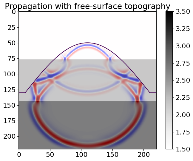
This notebook demonstrates the use of immersed boundary support (via Schism) to implement a topographic free surface.
Read the SDF
The boundary geometry in Schism is represented via a discretised signed distance function (SDF). To save computation when calculating the SDF, it only need to be calculated to a radius of space_order*max(spacing) from the surface. The interior region should be flood-filled to the radius chosen (this is necessary for interior-exterior sectioning).
Material properties should be continued through the surface; the immersed boundary imposes the free-surface condition explicitly, so there is no need to impose it implicitly with a material contrast. Furthermore, this avoids the risk of misalignment between the SDF and material contrast.
This demonstration SDF is for a simple sinusoid hill test surface. It is discretised on a 1km x 1km grid with 5m spacing. At the domain edge, SDFs should be extruded into the padding region as with any other material parameter. Recipes immersed boundary functionality assumes that the z axis points downwards.
sdf = np.load("test_surface_sdf.npy")

# Plotting the SDF
plt.imshow(sdf.T)
plt.colorbar()
# Plot the isosurface encapsulated by the SDF
plt.contour(sdf.T, [0])
plt.title("Surface SDF")
plt.show()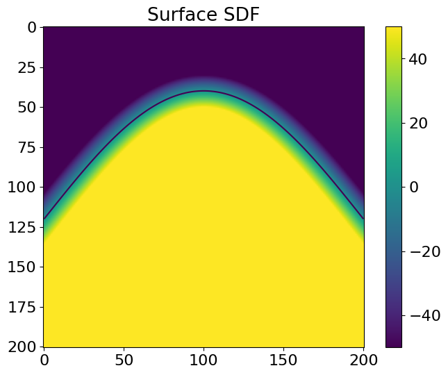
Set up the model and solver
The SDF is supplied in the same manner as material parameters. If an SDF is supplied, then an immersed boundary is automatically set up.
physics = 'iso-acoustic'
kwargs = {'shape': (201, 201), 'spacing': (5., 5.), 'space_order': 4,
          'nt': 250, 'f0': 0.040, 'sdf': sdf}

model = layered_model(physics, **kwargs)

solver = recipes_registry[physics](model, kwargs)

center = (np.array(model.shape) - 1)*np.array(model.spacing)/2
solver.src.coordinates.data[:] = center
Operator `initdamp` ran in 0.01 ssolver.forward()Operator `normals` ran in 0.01 sGenerating stencils for Derivative(u(t, x, y), (x, 2))
Generating stencils for Derivative(u(t, x, y), (y, 2))Operator `ForwardAcousticIsotropic` ran in 0.07 sPerformanceSummary([(PerfKey(name='section0', rank=None),
PerfEntry(time=0.00014199999999999998, gflopss=0.0, gpointss=0.0, oi=0.0, ops=0, itershapes=[])),
(PerfKey(name='section1', rank=None),
PerfEntry(time=9.999999999999999e-05, gflopss=0.0, gpointss=0.0, oi=0.0, ops=0, itershapes=[])),
(PerfKey(name='section2', rank=None),
PerfEntry(time=8.999999999999999e-05, gflopss=0.0, gpointss=0.0, oi=0.0, ops=0, itershapes=[])),
(PerfKey(name='section3', rank=None),
PerfEntry(time=0.027496000000000003, gflopss=0.0, gpointss=0.0, oi=0.0, ops=0, itershapes=[])),
(PerfKey(name='section4', rank=None),
PerfEntry(time=0.015969999999999995, gflopss=0.0, gpointss=0.0, oi=0.0, ops=0, itershapes=[])),
(PerfKey(name='section5', rank=None),
PerfEntry(time=0.00441, gflopss=0.0, gpointss=0.0, oi=0.0, ops=0, itershapes=[])),
(PerfKey(name='section6', rank=None),
PerfEntry(time=1e-06, gflopss=0.0, gpointss=0.0, oi=0.0, ops=0, itershapes=[])),
(PerfKey(name='section7', rank=None),
PerfEntry(time=1e-06, gflopss=0.0, gpointss=0.0, oi=0.0, ops=0, itershapes=[])),
(PerfKey(name='section8', rank=None),
PerfEntry(time=1e-06, gflopss=0.0, gpointss=0.0, oi=0.0, ops=0, itershapes=[])),
(PerfKey(name='section9', rank=None),
PerfEntry(time=0.016209000000000008, gflopss=0.0, gpointss=0.0, oi=0.0, ops=0, itershapes=[]))])plt.imshow(model.vp.data.T, cmap='Greys')
plt.colorbar()
pressure = solver.pressure.data[-1]
vmax = np.amax(np.abs(pressure))
plt.imshow(pressure.T, cmap='seismic', alpha=0.5,
vmin=-vmax, vmax=vmax)
# Plot sdf isosurface
plt.contour(model.sdf.data.T, [0])
plt.title("Propagation with free-surface topography")
plt.show()