import numpy as np
from devito import Constant
from recipes import WaveModel, AcousticIsotropic
import matplotlib.pyplot as pltAttenuation with SLS
In this notebook, we show the effect of attenuation (Qp) in a constant medium, showing the phase and amplitude alteration of the wavefield. This notebook also serves as a visual validation of our implementation showing standard plots from the literature.
We first setup the domain and constant model
shape = (501, 501)
nbl = 0
space_order = 8
spacing = (10., 10.)
origin = (0., 0.)
vp = 2.5 # 1.5 km/s
invqp = Constant(name="invqp", value=1/100) #
model = WaveModel(origin, spacing, shape, space_order, vp, nbl=nbl, b=1, invqp=invqp, dt=1.0)
model.physical_parameters('vp', 'b', 'invqp')We now setup the solve
solver = AcousticIsotropic(model, {'nt': 500})

# Put the source in the middle
solver.src.coordinates.data[0, :] = np.array(model.domain_size) * .5
Attenuation effect
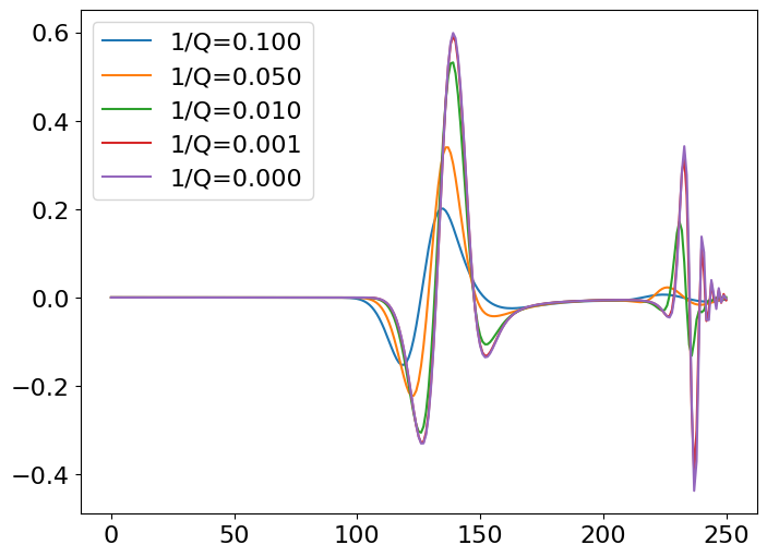
We compute the response of the media for multiple values of Q 10, 20, 100, 1000, Inf and expect the attenuation effect to reduce with higher values while lower values will shot more pronounced effects on the phase and amplitude of the wavefield
invQ = [1/10, 1/20, 1/100, 1/1000, 0]

traces = []
plt.figure(figsize=(10, 10))

for (i, iq) in enumerate(invQ):
    model.invqp.data = iq
    solver.forward(nt=498)
    traces.append(solver.state['u'].data[0, :251, 231].copy())
    plt.subplot(3, 2, i+1)
    plt.imshow(solver.state['u'].data[0, :, :].T, cmap='seismic', vmin=-.1, vmax=.1)
    plt.title('1/Q = %2.3f' %iq)
plt.tight_layout()
Operator `ForwardAcousticIsotropic` ran in 0.37 s
Operator `ForwardAcousticIsotropic` ran in 0.27 s
Operator `ForwardAcousticIsotropic` ran in 0.32 s
Operator `ForwardAcousticIsotropic` ran in 0.67 s
Operator `ForwardAcousticIsotropic` ran in 0.61 s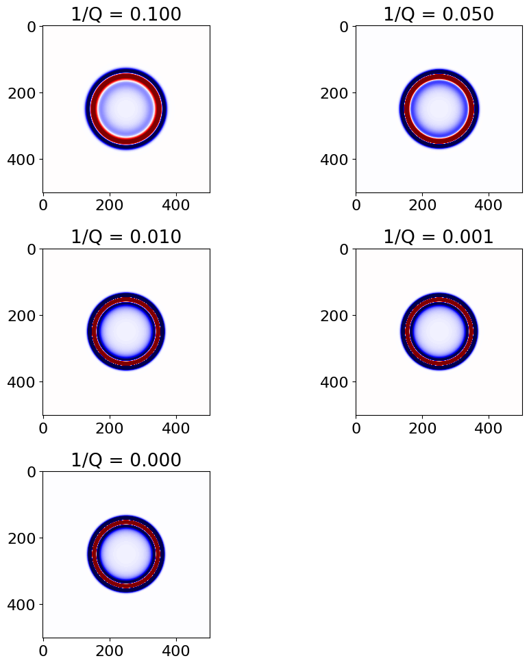
plt.figure()
for i, iq in enumerate(invQ):
    plt.plot(traces[i], label='1/Q=%2.3f' % iq)
plt.legend()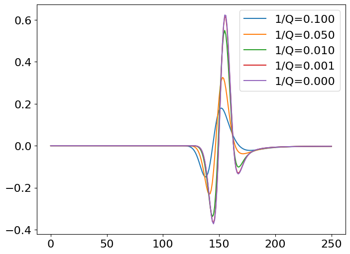
As expected we see the effect of attenuation on the phase and amplitude of the wavefield. The effect is more pronounced for lower values of Q and reduces with higher values of Q. This result matches the expected behavior of attenuation with a single SLS memory variable as in e.g Blanch and Symes.
Anisotropic equation
We follow this isotropic acoustic example by doing the same analysis in an anisotropic acoustic medium. We first show that by setting the Thomsen parameter to 0, we recover the isotropic case then we show we obtain similar behavior with a VTI configuration.
We only support attenuation in a VTI/TTI model through the Zhang formulation (see Zhang et al.). The Fletcher could support it in a smiliar way but we chose to use the formulation demnstrated to be more stable w.r.t strong anisotropy heterogeneity. Concerning the self-adjoint formulation, a new phase-velocity equivalent derivation taking the SLS relaxation into account is required.
from recipes import ZhangTTI

epsilon = 0
delta = 0

model = WaveModel(origin, spacing, shape, space_order, vp, nbl=nbl, b=1, epsilon=epsilon, delta=delta, dt=1.0, invqp=invqp)
solver = ZhangTTI(model, {'nt': 500})
# Put the source in the middle
solver.src.coordinates.data[0, :] = np.array(model.domain_size) * .5traces = []
plt.figure(figsize=(10, 10))
for (i, iq) in enumerate(invQ):
model.invqp.data = iq
solver.forward(nt=498)
traces.append(solver.state['u'].data[0, :251, 231].copy())
plt.subplot(3, 2, i+1)
plt.imshow(solver.state['u'].data[0, :, :].T, cmap='seismic', vmin=-.1, vmax=.1)
plt.title('1/Q = %2.3f' %iq)
plt.tight_layout()Operator `ForwardZhangTTI` ran in 0.41 s
Operator `ForwardZhangTTI` ran in 0.28 s
Operator `ForwardZhangTTI` ran in 0.20 s
Operator `ForwardZhangTTI` ran in 0.18 s
Operator `ForwardZhangTTI` ran in 0.19 s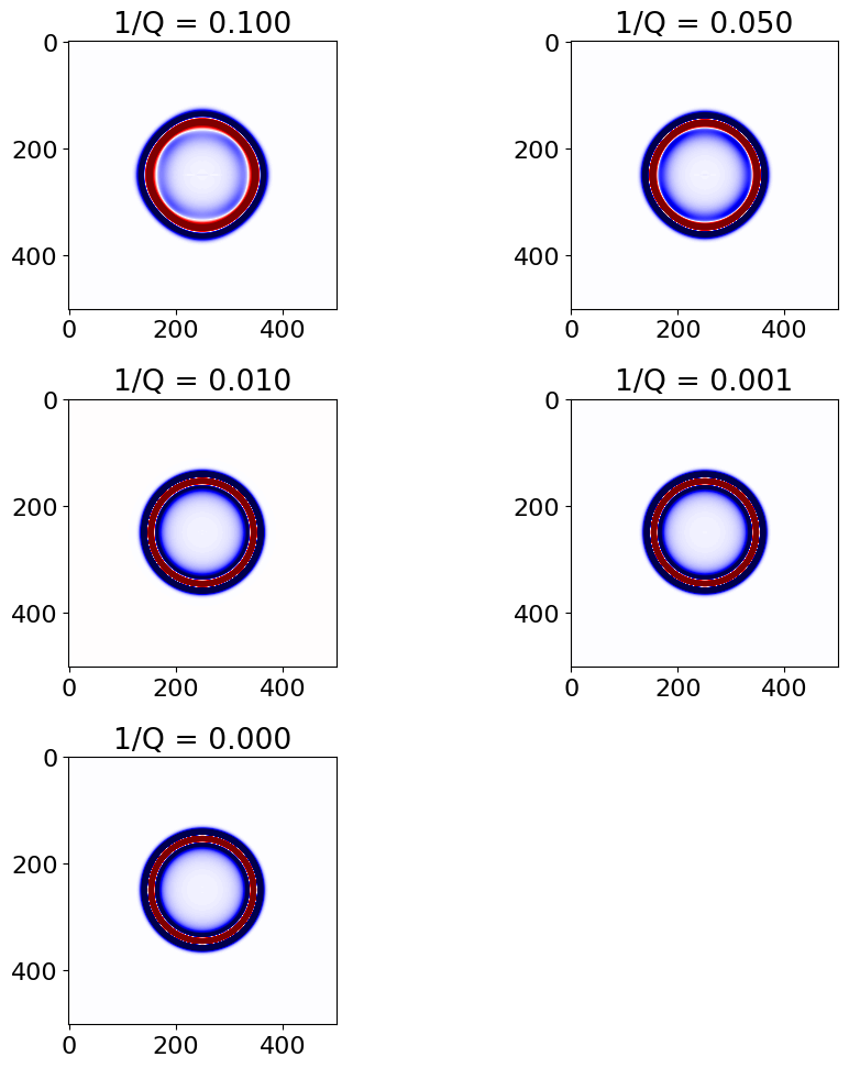
plt.figure()
for i, iq in enumerate(invQ):
plt.plot(traces[i], label='1/Q=%2.3f' % iq)
plt.legend()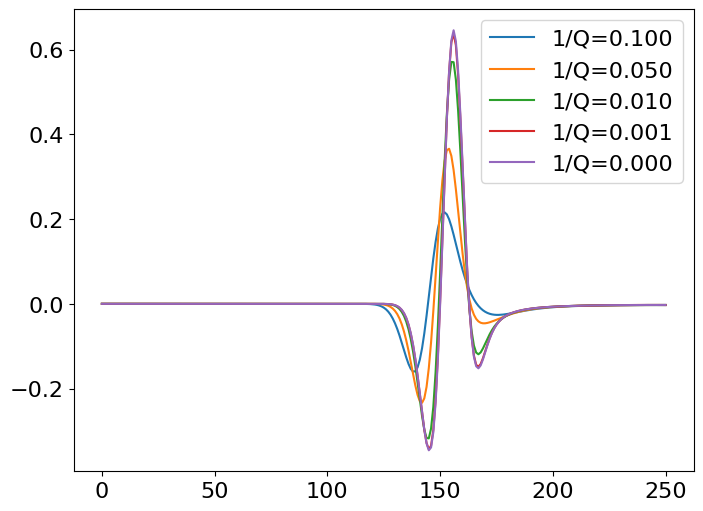
And we finally run it with anisotropy
model.epsilon.data = 0.2
model.delta.data = 0.05
traces = []

plt.figure(figsize=(10, 10))

for (i, iq) in enumerate(invQ):
    model.invqp.data = iq
    solver.forward(nt=498)
    traces.append(solver.state['u'].data[0, :251, 231].copy())
    plt.subplot(3, 2, i+1)
    plt.imshow(solver.state['u'].data[0, :, :].T, cmap='seismic', vmin=-.1, vmax=.1)
    plt.title('1/Q = %2.3f' %iq)
plt.tight_layout()
Operator `ForwardZhangTTI` ran in 0.26 s
Operator `ForwardZhangTTI` ran in 0.19 s
Operator `ForwardZhangTTI` ran in 0.19 s
Operator `ForwardZhangTTI` ran in 0.19 s
Operator `ForwardZhangTTI` ran in 0.19 s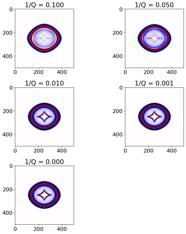
plt.figure()
for i, iq in enumerate(invQ):
    plt.plot(traces[i], label='1/Q=%2.3f' % iq)
plt.legend()