import devito
from devitopro import *
from examples.seismic import demo_model, setup_geometryDispersion minimization
We provide a brief overview of dispersion reduction FD schemes in devitopro. By default, devito automatically generates taylor based finite difference coefficients for all derivatives. However, thos finite difference coefficients are not always optimal. On way to improve the accuracy of the finite difference scheme is to minimize the dispersion error.
In devitopro the Taylor coefficents are replaced by dispersion minimizing coefficients providing higher accuracy wave modelling. We show in the following on a simple 2D model the adavantage of it.
Second order equation
Let’s make a simple layered model with a source at the top.
#NBVAL_IGNORE_OUTPUT

so = 8
model = demo_model('layers-isotropic', shape=(201, 201), spacing=(15., 15.), space_order=so, nbl=40)
geometry = setup_geometry(model, 1250, f0=0.015)
src = geometry.src
NUMA domain count autodetection failed, assuming 1
Operator `initdamp` ran in 0.01 sfrom examples.seismic import plot_velocity
plot_velocity(model, source=src.coordinates.data)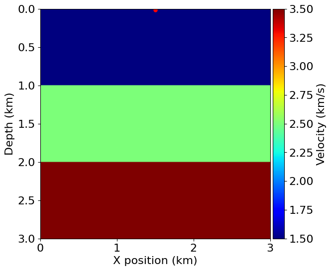
from devito import Eq, solve, Operator

u = devito.TimeFunction(name="u", grid=model.grid, space_order=so, time_order=2)
u_dr = TimeFunction(name="u_dr", grid=model.grid, space_order=so, time_order=2, coefficients="lsqr_drp")

eq = model.m * u.dt2 - u.laplace + model.damp * u.dt
eq_dr = model.m * u_dr.dt2 - u_dr.laplace + model.damp * u_dr.dt

stencil = Eq(u.forward, solve(eq, u.forward))
stencil_dr = Eq(u_dr.forward, solve(eq_dr, u_dr.forward))

srceq = src.inject((u_dr.forward, u.forward), expr=src)
Let’s first look t the finite difference coefficients for the second derivative.
u.dx2.evaluate\(\displaystyle - \frac{2.84722222 u(t, x, y)}{h_{x}^{2}} - \frac{0.00178571429 u(t, x - 4*h_x, y)}{h_{x}^{2}} + \frac{0.0253968254 u(t, x - 3*h_x, y)}{h_{x}^{2}} - \frac{0.2 u(t, x - 2*h_x, y)}{h_{x}^{2}} + \frac{1.6 u(t, x - h_x, y)}{h_{x}^{2}} + \frac{1.6 u(t, x + h_x, y)}{h_{x}^{2}} - \frac{0.2 u(t, x + 2*h_x, y)}{h_{x}^{2}} + \frac{0.0253968254 u(t, x + 3*h_x, y)}{h_{x}^{2}} - \frac{0.00178571429 u(t, x + 4*h_x, y)}{h_{x}^{2}}\)
#NBVAL_IGNORE_OUTPUT
u_dr.dx2.evaluate
\(\displaystyle - \frac{3.07581966 u_dr(t, x, y)}{h_{x}^{2}} - \frac{0.00811027728 u_dr(t, x - 4*h_x, y)}{h_{x}^{2}} + \frac{0.0641006396 u_dr(t, x - 3*h_x, y)}{h_{x}^{2}} - \frac{0.30972732 u_dr(t, x - 2*h_x, y)}{h_{x}^{2}} + \frac{1.79164664 u_dr(t, x - h_x, y)}{h_{x}^{2}} + \frac{1.79164664 u_dr(t, x + h_x, y)}{h_{x}^{2}} - \frac{0.30972732 u_dr(t, x + 2*h_x, y)}{h_{x}^{2}} + \frac{0.0641006396 u_dr(t, x + 3*h_x, y)}{h_{x}^{2}} - \frac{0.00811027728 u_dr(t, x + 4*h_x, y)}{h_{x}^{2}}\)
#NBVAL_IGNORE_OUTPUT

op = Operator([stencil, stencil_dr] + srceq)
summary = op(dt=model.critical_dt)
Operator `Kernel` ran in 0.07 sWe now look at the solution wavefield. We clearly see that the wavefield with the devitopro coefficients is much more accurate and drastically less dispersive. Those improvement are automatically applied to all finite difference coefficients unless explicitly turned off by specifying taylor coefficients
u_taylor = Function(name="u_taylor", grid=grid, space_order=space_order, coefficients='taylor')You can also explicitly specify the dispersion minimizing coefficients by using the lsqr_dr coefficients with devitpro.
u_lsqr = Function(name="u_lsqr", grid=grid, space_order=space_order, coefficients='lsqr_dr')#NBVAL_IGNORE_OUTPUT
import matplotlib.pyplot as plt
plt.figure(figsize=(12, 12))
plt.subplot(121)
plt.imshow(u.data[0].T, vmin=-.5, vmax=.5, cmap="seismic")
plt.title("Taylor FD")
plt.subplot(122)
plt.imshow(u_dr.data[0].T, vmin=-.5, vmax=.5, cmap="seismic")
plt.title("DevitoPro FD")Text(0.5, 1.0, 'DevitoPro FD')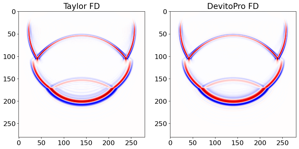
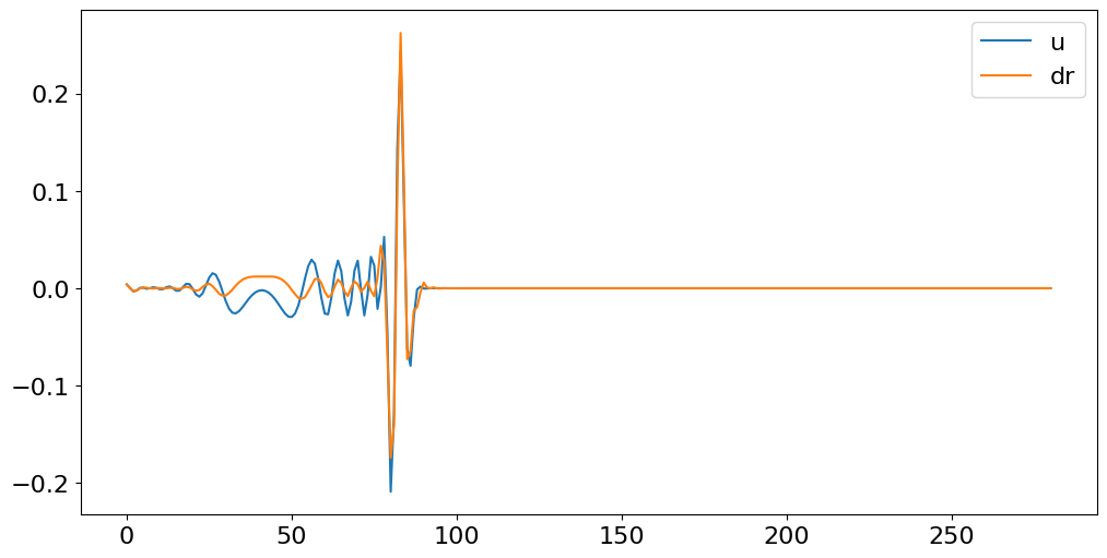
#NBVAL_IGNORE_OUTPUT

plt.figure(figsize=(12, 6))
plt.plot(u.data[0, 100, :], label="u")
plt.plot(u_dr.data[0, 100, :], label="dr")
plt.legend()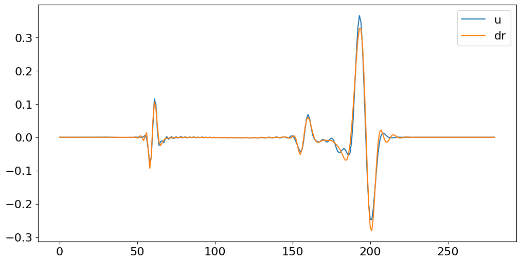
First order equation
We now show that those improvements are also available for first order equations such as the first order acoustic isotropic wave equation
from devito import grad, div, NODE

u = devito.TimeFunction(name="u", grid=model.grid, space_order=so, time_order=1, staggered=NODE)
u_dr = TimeFunction(name="u_dr", grid=model.grid, space_order=so, time_order=1, staggered=NODE, coefficients="lsqr_drp")

v = devito.VectorTimeFunction(name="v", grid=model.grid, space_order=so, time_order=1)
v_dr = VectorTimeFunction(name="v_dr", grid=model.grid, space_order=so, time_order=1, coefficients="lsqr_drp")

ro = 1
l2m = 1 / model.m
mask = 1 - model.damp

# The source injection term
geometry = setup_geometry(model, 1250, f0=0.010)
src = geometry.src
src_p = src.inject(field=(u.forward, u_dr.forward), expr=src)

# First order equations
u_v = Eq(v.forward, mask * solve(v.dt - ro * grad(u), v.forward))
u_p = Eq(u.forward, mask * solve(u.dt - l2m * div(v.forward), u.forward))

u_v_dr = Eq(v_dr.forward, mask * solve(v_dr.dt - ro * grad(u_dr), v_dr.forward))
u_p_dr = Eq(u_dr.forward, mask * solve(u_dr.dt - l2m * div(v_dr.forward), u_dr.forward))
#NBVAL_IGNORE_OUTPUT
op = Operator([u_v, u_p, u_v_dr, u_p_dr] + src_p)
op(dt=model.critical_dt/2)Operator `Kernel` ran in 0.14 sPerformanceSummary([(PerfKey(name='section0', rank=None),
PerfEntry(time=0.0928140000000001, gflopss=0.0, gpointss=0.0, oi=0.0, ops=0, itershapes=[])),
(PerfKey(name='section1', rank=None),
PerfEntry(time=0.032416, gflopss=0.0, gpointss=0.0, oi=0.0, ops=0, itershapes=[])),
(PerfKey(name='section2', rank=None),
PerfEntry(time=0.004718000000000014, gflopss=0.0, gpointss=0.0, oi=0.0, ops=0, itershapes=[]))])#NBVAL_IGNORE_OUTPUT
plt.figure(figsize=(12, 12))
plt.subplot(121)
plt.imshow(u.data[0].T, vmin=-.5, vmax=.5, cmap="seismic")
plt.title("Taylor FD")
plt.subplot(122)
plt.imshow(u_dr.data[0].T, vmin=-.5, vmax=.5, cmap="seismic")
plt.title("DevitoPro FD")Text(0.5, 1.0, 'DevitoPro FD')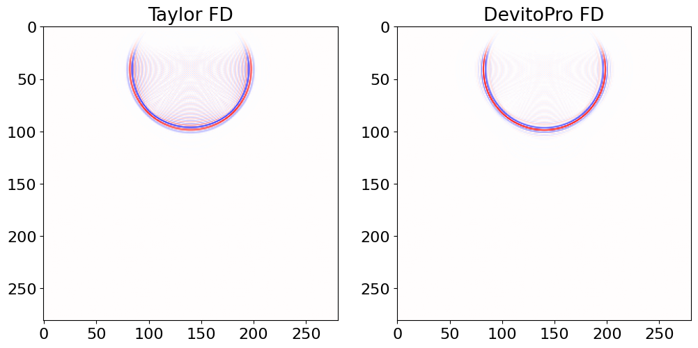
#NBVAL_IGNORE_OUTPUT

plt.figure(figsize=(12, 6))
plt.plot(u.data[0, 100, :], label="u")
plt.plot(u_dr.data[0, 100, :], label="dr")
plt.legend()