import os
os.environ['DEVITO_LOGGING'] = 'ERROR'
os.environ['OMP_NUM_THREADS'] =  str(os.cpu_count() // 2)

import urllib.request
import zipfile
import globSEAM Elastic 2D Tutorial
This tutorial demonstrates the full workflow for setting up an elastic wave propagation simulation and computing a single-shot gradient using a real-world model. We use the SEAM Phase I 2D elastic model and the pysegy library for SEG-Y I/O.
The workflow covers: 1. Downloading and reading the SEAM 2D model from SEG-Y files 2. Building a WaveModel from the loaded arrays 3. Creating a solver and running a forward simulation 4. Computing a single-shot gradient via the adjoint-state method
import numpy as np
import matplotlib.pyplot as plt

from pysegy import segy_read, get_header
from pysegy.plotting import plot_velocity, plot_sdata, plot_simage

from examples.seismic import Receiver
from recipes import recipes_registry
from recipes.model import WaveModel
1. Download the SEAM 2D model
The SEAM Phase I 2D elastic model is publicly available as a zip archive. We download and extract it into a local directory.
url = "https://seam-open-data.s3.us-west-2.amazonaws.com/Phase+I/SEAM_I_2D_Model.zip"
zip_path = "SEAM_I_2D_Model.zip"
extract_dir = "SEAM_I_2D_Model"

if not os.path.isdir(extract_dir):
    if not os.path.isfile(zip_path):
        print("Downloading SEAM 2D model...")
        urllib.request.urlretrieve(url, zip_path)
        print("Download complete.")
    print("Extracting...")
    with zipfile.ZipFile(zip_path, 'r') as zf:
        zf.extractall(extract_dir)
    print("Extraction complete.")
else:
    print(f"Directory '{extract_dir}' already exists, skipping download.")
Directory 'SEAM_I_2D_Model' already exists, skipping download.# List the extracted files
for root, dirs, files in os.walk(extract_dir):
for f in sorted(files):
fpath = os.path.join(root, f)
size_mb = os.path.getsize(fpath) / 1e6
print(f" {fpath} ({size_mb:.1f} MB)") SEAM_I_2D_Model/SEAM_I_2D_Model/LICENSE TO SEAM OPEN DATA.pdf (0.0 MB)
SEAM_I_2D_Model/SEAM_I_2D_Model/SEAM_2D_Model_Subset.pdf (0.0 MB)
SEAM_I_2D_Model/SEAM_I_2D_Model/SEAM_2D_Model_Subset_plots.pdf (0.9 MB)
SEAM_I_2D_Model/SEAM_I_2D_Model/SEAM_Den_Elastic_N23900.sgy (10.9 MB)
SEAM_I_2D_Model/SEAM_I_2D_Model/SEAM_Vp_Elastic_N23900.sgy (10.9 MB)
SEAM_I_2D_Model/SEAM_I_2D_Model/SEAM_Vs_Elastic_N23900.sgy (10.9 MB)2. Read the model from SEG-Y
The SEAM 2D model ships as SEG-Y files for Vp, Vs, and density. We read each file with pysegy.segy_read which returns a SeisBlock. The grid spacing is extracted from the headers:
- dz from the binary file header sample interval (
bfh.dt, in micrometers for depth models) - dx from the difference in
CDPXcoordinates between consecutive traces
# Find the SEG-Y files in the extracted directory
segy_files = sorted(
    glob.glob(os.path.join(extract_dir, '**', '*.segy'), recursive=True)
    + glob.glob(os.path.join(extract_dir, '**', '*.sgy'), recursive=True)
)
for f in segy_files:
    print(f)
SEAM_I_2D_Model/SEAM_I_2D_Model/SEAM_Den_Elastic_N23900.sgy
SEAM_I_2D_Model/SEAM_I_2D_Model/SEAM_Vp_Elastic_N23900.sgy
SEAM_I_2D_Model/SEAM_I_2D_Model/SEAM_Vs_Elastic_N23900.sgydef read_segy_model(filepath):
"""Read a SEG-Y model file and return the data, dx, and dz."""
block = segy_read(filepath)
# dz from the binary file header sample interval
dz = block.fileheader.bfh.dt / 1000
# dx from the CDPX coordinate difference between first two traces
dx = np.diff(get_header(block.traceheaders[:2], 'SourceX'))[0]
# Each trace is one x-position with nz depth samples,
# so np.array gives (ntraces, nsamples) = (nz, nx).
# Transpose to (nx, nz) for WaveModel.
data = np.array(block.data).T
print(f" {os.path.basename(filepath)}: "
f"shape {data.shape} (nx, nz), dx={dx} m, dz={dz} m")
return data, dx, dz# Read Vp, Vs and density
vp_data, vs_data, rho_data = None, None, None
dx, dz = None, None
for fp in segy_files:
name = os.path.basename(fp).lower()
if 'vp' in name or 'pwave' in name:
print("Reading Vp:")
vp_data, dx, dz = read_segy_model(fp)
elif 'vs' in name or 'swave' in name:
print("Reading Vs:")
vs_data, _, _ = read_segy_model(fp)
elif 'rho' in name or 'den' in name:
print("Reading density:")
rho_data, _, _ = read_segy_model(fp)
print(f"\nGrid spacing from headers: dx={dx} m, dz={dz} m")Reading density:
SEAM_Den_Elastic_N23900.sgy: shape (1751, 1501) (nx, nz), dx=20 m, dz=10.0 m
Reading Vp:
SEAM_Vp_Elastic_N23900.sgy: shape (1751, 1501) (nx, nz), dx=20 m, dz=10.0 m
Reading Vs:
SEAM_Vs_Elastic_N23900.sgy: shape (1751, 1501) (nx, nz), dx=20 m, dz=10.0 m
Grid spacing from headers: dx=20 m, dz=10.0 mprint(f"Vp shape: {vp_data.shape}, "
f"range: [{vp_data.min():.1f}, {vp_data.max():.1f}]")
print(f"Vs shape: {vs_data.shape}, "
f"range: [{vs_data.min():.1f}, {vs_data.max():.1f}]")
print(f"Rho shape: {rho_data.shape}, "
f"range: [{rho_data.min():.1f}, {rho_data.max():.1f}]")Vp shape: (1751, 1501), range: [1490.0, 4800.0]
Vs shape: (1751, 1501), range: [0.0, 2965.5]
Rho shape: (1751, 1501), range: [1.0, 2.7]3. Prepare the model arrays
The SEAM model uses SI units (m/s for velocity, kg/m³ for density). The recipes package expects velocity in km/s and buoyancy b = 1/rho. The grid spacing was extracted from the SEG-Y headers above.
We subsample the model for a faster demonstration.
# Convert from m/s to km/s
vp_km = vp_data.astype(np.float32) / 1000.0
vs_km = vs_data.astype(np.float32) / 1000.0
rho = rho_data.astype(np.float32)

# Subsample in x and z
subx, subz = 2, 4
vp_sub = vp_km[::subx, ::subz]
vs_sub = vs_km[::subx, ::subz]
rho_sub = rho[::subx, ::subz]

# Buoyancy
b_sub = 1.0 / rho_sub

# Grid spacing after subsampling in x
dx_sub = dx * subx
dz_sub = dz * subz

shape = vp_sub.shape
print(f"Subsampled shape: {shape} (nx, nz)")
print(f"Grid spacing: dx={dx_sub} m, dz={dz_sub} m")
print(f"Physical extent: "
      f"{(shape[0]-1)*dx_sub:.0f} m x {(shape[1]-1)*dz_sub:.0f} m")
Subsampled shape: (876, 376) (nx, nz)
Grid spacing: dx=40 m, dz=40.0 m
Physical extent: 35000 m x 15000 mPlot the model
spacing = (dz_sub, dx_sub)

plt.figure(figsize=(18, 5))
plt.subplot(1, 3, 1)
plot_velocity(vp_sub.T, spacing=spacing,
              name='P-wave velocity (km/s)', cbar=True, new_fig=False)
plt.subplot(1, 3, 2)
plot_velocity(vs_sub.T, spacing=spacing,
              name='S-wave velocity (km/s)', cbar=True, new_fig=False)
plt.subplot(1, 3, 3)
plot_velocity(rho_sub.T, spacing=spacing,
              name='Density (kg/m\u00b3)', cbar=True, new_fig=False)
plt.tight_layout()
plt.show()
Detect the ocean bottom for OBN acquisition
For an Ocean Bottom Node (OBN) survey, receivers sit on the sea floor. We detect the water bottom from the Vs model: in the water column Vs is zero (or negligible), so the first depth index where Vs exceeds a small threshold gives the sea-floor depth at each x position.
# Detect the water bottom depth at each x position from Vs
# In the water column Vs ~ 0; the sea floor is where Vs first
# exceeds a small threshold.
vs_threshold = 0.01  # km/s
wb_indices = np.argmax(vs_sub > vs_threshold, axis=1)

# Convert grid indices to physical depth (m)
wb_depth = wb_indices * dz_sub

# OBN receiver spacing
rec_spacing = 50.0  # m
x_extent = (shape[0] - 1) * dx_sub
rec_x = np.arange(rec_spacing, x_extent - rec_spacing / 2,
                   rec_spacing)
nrec = len(rec_x)

# Interpolate the water-bottom depth at each receiver x position
x_grid = np.arange(shape[0]) * dx_sub
rec_z = np.interp(rec_x, x_grid, wb_depth) - 50.0

print(f"Number of OBN receivers: {nrec}")
print(f"Receiver x range: [{rec_x[0]:.0f}, {rec_x[-1]:.0f}] m")
print(f"Water bottom depth range: "
      f"[{rec_z.min():.0f}, {rec_z.max():.0f}] m")
Number of OBN receivers: 699
Receiver x range: [50, 34950] m
Water bottom depth range: [710, 1590] m# Plot the OBN receiver positions on top of the Vs model
plot_velocity(vs_sub.T, spacing=spacing,
name='OBN receiver layout on Vs model',
cbar=True)
plt.plot(rec_x, rec_z, 'wv', markersize=4, label='OBN receivers')
plt.legend(loc='lower right')
plt.tight_layout()
plt.show()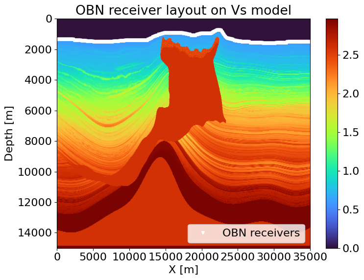
4. Build the WaveModel
We construct a WaveModel directly from the arrays. For elastic modeling we pass vp and vs; the model internally computes the Lame parameters lam and mu.
nbl = 40     # absorbing boundary width
so = 8       # spatial finite-difference order

model = WaveModel(
    origin=(0.0, 0.0),
    spacing=(dx_sub, dz_sub),
    shape=shape,
    space_order=so,
    vp=vp_sub,
    vs=vs_sub,
    b=b_sub,
    nbl=nbl,
    fs=True,
    dtype=np.float32,
)

print(f"Model shape (with boundary): {model.grid.shape}")
print(f"CFL time step: {model.critical_dt:.4f} ms")
Model shape (with boundary): (np.int64(956), np.int64(416))
CFL time step: 4.3520 ms5. Create the solver and set up OBN acquisition
We use the iso-elastic solver from the registry. The source is a Ricker wavelet injected into the stress diagonal. For OBN acquisition the receivers are placed every 50 m along the ocean bottom, which we detected from the Vs model above.
Because the default solver creates its own receiver array, we build a custom Receiver object with the OBN coordinates and assign it to the solver before running the forward pass.
# Simulation parameters
t_end = 10000.0  # total simulation time in ms
nt = int(t_end / model.critical_dt) + 1
f0 = 0.005      # dominant frequency in kHz (10 Hz)

options = {
    'space_order': so,
    'nt': nt,
    'f0': f0,
    't_sub': 5, # Time subsampling factor (save every t_sub steps)
    'save': None,
    'compression': True, # Will pick cvxcompress or bitcomp based on platform
    'save': 'lazy'
}

solver = recipes_registry['iso-elastic'](model, options)

# Build OBN receiver coordinates array (nrec, 2)
rec_coords = np.zeros((nrec, 2), dtype=np.float32)
rec_coords[:, 0] = rec_x
rec_coords[:, 1] = rec_z

# Replace the default receiver with OBN geometry
solver.rec = Receiver(
    name='rec', grid=solver.grid, npoint=nrec,
    time_range=solver.src.time_range,
    coordinates=rec_coords,
)

print(f"Number of time steps: {nt}")
print(f"Total simulation time: {nt * model.critical_dt:.1f} ms")
print(f"Source frequency: {f0 * 1e3:.0f} Hz")
print(f"OBN receivers: {nrec} nodes, "
      f"spacing {rec_spacing:.0f} m")
Number of time steps: 2298
Total simulation time: 10000.9 ms
Source frequency: 5 Hz
OBN receivers: 699 nodes, spacing 50 m# Position the source at the surface, center of the model
src = solver.src
src.coordinates.data[0, 0] = (shape[0] - 1) * dx_sub / 3
src.coordinates.data[0, -1] = 1.25 * dz_sub
print(f"Source position: "
f"x={src.coordinates.data[0, 0]:.0f} m, "
f"z={src.coordinates.data[0, -1]:.1f} m")
print(f"Number of OBN receivers: {nrec}")Source position: x=11667 m, z=50.0 m
Number of OBN receivers: 699# Plot the source wavelet
time_ms = np.arange(nt) * model.critical_dt
plt.figure(figsize=(10, 3))
plt.plot(time_ms, src.data[:, 0])
plt.xlabel('Time (ms)')
plt.ylabel('Amplitude')
plt.title('Ricker source wavelet')
plt.xlim(0, min(1500, time_ms[-1]))
plt.tight_layout()
plt.show()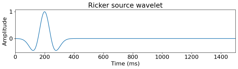
6. Forward simulation
Run the forward propagation to generate synthetic shot data.
summary = solver.forward()
print(summary)
PerformanceSummary({PerfKey(name='section0', rank=None): PerfEntry(time=0.000593, gflopss=0.0, gpointss=0.0, oi=0.0, ops=0, itershapes=[]), PerfKey(name='section1', rank=None): PerfEntry(time=1.8000010000000046, gflopss=0.0, gpointss=0.0, oi=0.0, ops=0, itershapes=[]), PerfKey(name='section2', rank=None): PerfEntry(time=0.08265300000000006, gflopss=0.0, gpointss=0.0, oi=0.0, ops=0, itershapes=[]), PerfKey(name='section3', rank=None): PerfEntry(time=0.10894799999999967, gflopss=0.0, gpointss=0.0, oi=0.0, ops=0, itershapes=[]), PerfKey(name='section4', rank=None): PerfEntry(time=0.105945, gflopss=0.0, gpointss=0.0, oi=0.0, ops=0, itershapes=[])})plt.figure(figsize=(15, 6))
plot_simage(solver.pressure_data.T, spacing=spacing, cmap="seismic",
name='Pressure', cbar=True, new_fig=False)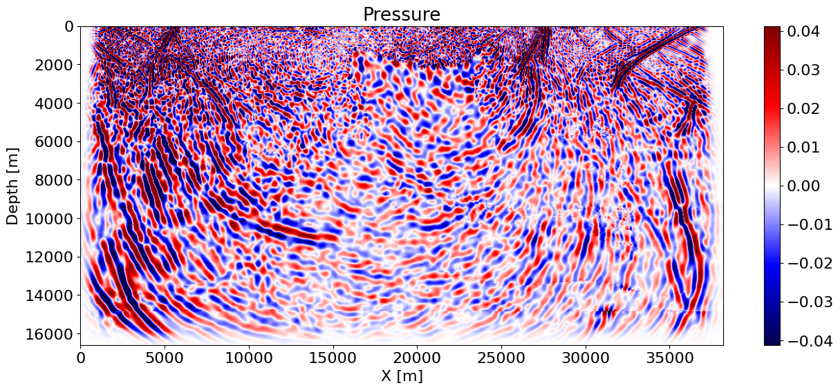
# Plot the shot record
true_data = solver.rec.data.copy()
dt_s = model.critical_dt / 1000  # ms -> s
rec_sp = (dt_s, rec_spacing)

plot_sdata(true_data, spacing=rec_sp, cmap='seismic',
           name='OBN shot record (true model)', perc=98)
plt.tight_layout()
plt.show()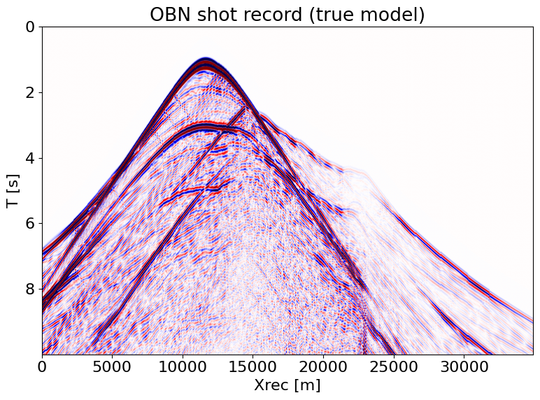
7. Compute a single-shot gradient
The gradient is computed via the adjoint-state method:
- Build a smooth background model
- Run the forward pass in the background model with wavefield saving
- Compute data residuals (background - true)
- Back-propagate the residuals and cross-correlate with the saved forward wavefield
The gradient images show where the model needs to be updated to reduce the data misfit.
from scipy.ndimage import gaussian_filter

# Create a smooth background model
sigma = 20  # smoothing radius in grid points
vp_smooth = gaussian_filter(vp_sub, sigma=sigma)
vs_smooth = gaussian_filter(vs_sub, sigma=sigma)
b_smooth = gaussian_filter(b_sub, sigma=sigma)

model0 = WaveModel(
    origin=(0.0, 0.0),
    spacing=(dx_sub, dz_sub),
    shape=shape,
    space_order=so,
    vp=vp_smooth,
    vs=vs_smooth,
    b=b_smooth,
    nbl=nbl,
    fs=True,
    dtype=np.float32,
    dt=model.critical_dt,
)

# Plot true vs smooth Vp
plt.figure(figsize=(14, 4))
plt.subplot(1, 2, 1)
plot_velocity(vp_sub.T, spacing=spacing,
              name='True Vp (km/s)', cbar=True, new_fig=False)
plt.subplot(1, 2, 2)
plot_velocity(vp_smooth.T, spacing=spacing,
              name='Smooth Vp (km/s)', cbar=True, new_fig=False)
plt.tight_layout()
plt.show()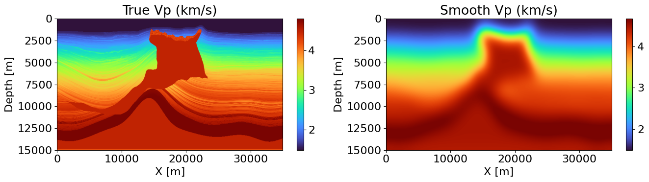
# Forward pass in the smooth model with wavefield saving
solver0 = recipes_registry['iso-elastic'](model0, options)

# Set the same source position
solver0.src.coordinates.data[:] = solver.src.coordinates.data[:]

# Use the same OBN receiver geometry
solver0.rec = Receiver(
    name='rec', grid=solver0.grid, npoint=nrec,
    time_range=solver0.src.time_range,
    coordinates=rec_coords.copy(),
)

solver0.forward(save=True)
PerformanceSummary([(PerfKey(name='section0', rank=None),
PerfEntry(time=0.0010479999999999999, gflopss=0.0, gpointss=0.0, oi=0.0, ops=0, itershapes=[])),
(PerfKey(name='section1', rank=None),
PerfEntry(time=0.000794, gflopss=0.0, gpointss=0.0, oi=0.0, ops=0, itershapes=[])),
(PerfKey(name='section2', rank=None),
PerfEntry(time=6.393791999999992, gflopss=0.0, gpointss=0.0, oi=0.0, ops=0, itershapes=[])),
(PerfKey(name='section3', rank=None),
PerfEntry(time=0.005523000000000128, gflopss=0.0, gpointss=0.0, oi=0.0, ops=0, itershapes=[])),
(PerfKey(name='section4', rank=None),
PerfEntry(time=0.028986999999999978, gflopss=0.0, gpointss=0.0, oi=0.0, ops=0, itershapes=[])),
(PerfKey(name='section5', rank=None),
PerfEntry(time=4e-06, gflopss=0.0, gpointss=0.0, oi=0.0, ops=0, itershapes=[])),
(PerfKey(name='section6', rank=None),
PerfEntry(time=0.6059270000000004, gflopss=0.0, gpointss=0.0, oi=0.0, ops=0, itershapes=[])),
(PerfKey(name='section7', rank=None),
PerfEntry(time=0.00022299999999999997, gflopss=0.0, gpointss=0.0, oi=0.0, ops=0, itershapes=[])),
(PerfKey(name='section8', rank=None),
PerfEntry(time=0.03579000000000003, gflopss=0.0, gpointss=0.0, oi=0.0, ops=0, itershapes=[])),
(PerfKey(name='section9', rank=None),
PerfEntry(time=6.999999999999999e-06, gflopss=0.0, gpointss=0.0, oi=0.0, ops=0, itershapes=[])),
(PerfKey(name='section10', rank=None),
PerfEntry(time=0.6238540000000002, gflopss=0.0, gpointss=0.0, oi=0.0, ops=0, itershapes=[])),
(PerfKey(name='section11', rank=None),
PerfEntry(time=1.2000000000000002e-05, gflopss=0.0, gpointss=0.0, oi=0.0, ops=0, itershapes=[])),
(PerfKey(name='section12', rank=None),
PerfEntry(time=0.028066999999999995, gflopss=0.0, gpointss=0.0, oi=0.0, ops=0, itershapes=[])),
(PerfKey(name='section13', rank=None),
PerfEntry(time=1.3000000000000003e-05, gflopss=0.0, gpointss=0.0, oi=0.0, ops=0, itershapes=[])),
(PerfKey(name='section14', rank=None),
PerfEntry(time=0.6386030000000004, gflopss=0.0, gpointss=0.0, oi=0.0, ops=0, itershapes=[])),
(PerfKey(name='section15', rank=None),
PerfEntry(time=1e-05, gflopss=0.0, gpointss=0.0, oi=0.0, ops=0, itershapes=[])),
(PerfKey(name='section16', rank=None),
PerfEntry(time=0.028212000000000015, gflopss=0.0, gpointss=0.0, oi=0.0, ops=0, itershapes=[])),
(PerfKey(name='section17', rank=None),
PerfEntry(time=1.3000000000000003e-05, gflopss=0.0, gpointss=0.0, oi=0.0, ops=0, itershapes=[])),
(PerfKey(name='section18', rank=None),
PerfEntry(time=0.6289819999999998, gflopss=0.0, gpointss=0.0, oi=0.0, ops=0, itershapes=[])),
(PerfKey(name='section19', rank=None),
PerfEntry(time=9e-06, gflopss=0.0, gpointss=0.0, oi=0.0, ops=0, itershapes=[])),
(PerfKey(name='section20', rank=None),
PerfEntry(time=0.02871599999999999, gflopss=0.0, gpointss=0.0, oi=0.0, ops=0, itershapes=[])),
(PerfKey(name='section21', rank=None),
PerfEntry(time=6.999999999999999e-06, gflopss=0.0, gpointss=0.0, oi=0.0, ops=0, itershapes=[])),
(PerfKey(name='section22', rank=None),
PerfEntry(time=0.6009660000000002, gflopss=0.0, gpointss=0.0, oi=0.0, ops=0, itershapes=[])),
(PerfKey(name='section23', rank=None),
PerfEntry(time=3.100000000000001e-05, gflopss=0.0, gpointss=0.0, oi=0.0, ops=0, itershapes=[])),
(PerfKey(name='section24', rank=None),
PerfEntry(time=0.04637800000000007, gflopss=0.0, gpointss=0.0, oi=0.0, ops=0, itershapes=[])),
(PerfKey(name='section25', rank=None),
PerfEntry(time=0.06184700000000036, gflopss=0.0, gpointss=0.0, oi=0.0, ops=0, itershapes=[]))])# Plot background shot record
bg_data = solver0.rec.data.copy()
plot_sdata(bg_data, spacing=rec_sp, cmap='seismic',
name='OBN shot record (smooth model)', perc=98)
plt.tight_layout()
plt.show()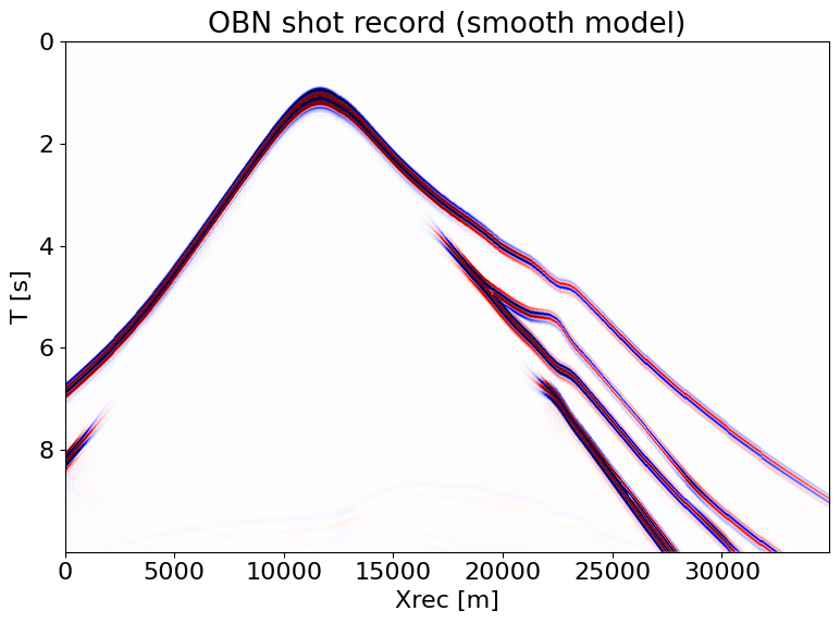
# Compute residuals and plot
residual = solver0.rec.data - true_data

plot_sdata(residual, spacing=rec_sp, cmap='seismic',
           name='Data residual (smooth - true)', perc=98)
plt.tight_layout()
plt.show()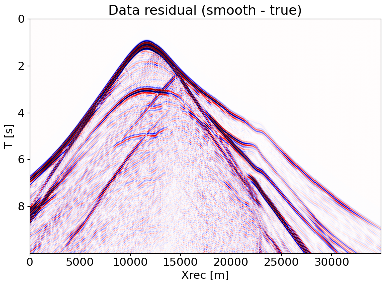
# Inject residuals and compute the gradient
solver0.rec.data[:] -= true_data
solver0.jacobian_adjoint(params=('vp', 'vs', 'b'))
PerformanceSummary([(PerfKey(name='section0', rank=None),
PerfEntry(time=0.017825, gflopss=0.0, gpointss=0.0, oi=0.0, ops=0, itershapes=[])),
(PerfKey(name='section1', rank=None),
PerfEntry(time=0.006546, gflopss=0.0, gpointss=0.0, oi=0.0, ops=0, itershapes=[])),
(PerfKey(name='section2', rank=None),
PerfEntry(time=6.150698000000006, gflopss=0.0, gpointss=0.0, oi=0.0, ops=0, itershapes=[])),
(PerfKey(name='section3', rank=None),
PerfEntry(time=0.24771799999999927, gflopss=0.0, gpointss=0.0, oi=0.0, ops=0, itershapes=[])),
(PerfKey(name='section4', rank=None),
PerfEntry(time=0.03456600000000025, gflopss=0.0, gpointss=0.0, oi=0.0, ops=0, itershapes=[])),
(PerfKey(name='section5', rank=None),
PerfEntry(time=0.44465099999999963, gflopss=0.0, gpointss=0.0, oi=0.0, ops=0, itershapes=[])),
(PerfKey(name='section6', rank=None),
PerfEntry(time=1.6000000000000003e-05, gflopss=0.0, gpointss=0.0, oi=0.0, ops=0, itershapes=[])),
(PerfKey(name='section7', rank=None),
PerfEntry(time=0.4269480000000005, gflopss=0.0, gpointss=0.0, oi=0.0, ops=0, itershapes=[])),
(PerfKey(name='section8', rank=None),
PerfEntry(time=3.3e-05, gflopss=0.0, gpointss=0.0, oi=0.0, ops=0, itershapes=[])),
(PerfKey(name='section9', rank=None),
PerfEntry(time=0.1987950000000002, gflopss=0.0, gpointss=0.0, oi=0.0, ops=0, itershapes=[])),
(PerfKey(name='section10', rank=None),
PerfEntry(time=0.41618499999999936, gflopss=0.0, gpointss=0.0, oi=0.0, ops=0, itershapes=[])),
(PerfKey(name='section11', rank=None),
PerfEntry(time=2.900000000000001e-05, gflopss=0.0, gpointss=0.0, oi=0.0, ops=0, itershapes=[])),
(PerfKey(name='section12', rank=None),
PerfEntry(time=0.29062299999999996, gflopss=0.0, gpointss=0.0, oi=0.0, ops=0, itershapes=[])),
(PerfKey(name='section13', rank=None),
PerfEntry(time=0.4218819999999998, gflopss=0.0, gpointss=0.0, oi=0.0, ops=0, itershapes=[])),
(PerfKey(name='section14', rank=None),
PerfEntry(time=1.3000000000000003e-05, gflopss=0.0, gpointss=0.0, oi=0.0, ops=0, itershapes=[])),
(PerfKey(name='section15', rank=None),
PerfEntry(time=0.42613099999999965, gflopss=0.0, gpointss=0.0, oi=0.0, ops=0, itershapes=[])),
(PerfKey(name='section16', rank=None),
PerfEntry(time=3.599999999999999e-05, gflopss=0.0, gpointss=0.0, oi=0.0, ops=0, itershapes=[])),
(PerfKey(name='section17', rank=None),
PerfEntry(time=0.4698699999999997, gflopss=0.0, gpointss=0.0, oi=0.0, ops=0, itershapes=[]))])# Remove boundary regions for plotting
z0 = 0 if model.fs else nbl
sl = np.s_[nbl:-nbl, z0:-nbl]
# Extract gradients
grad_vp = np.array(solver0.perturbation(param='vp').data)[sl]
grad_vs = np.array(solver0.perturbation(param='vs').data)[sl]
grad_b = np.array(solver0.perturbation(param='b').data)[sl]
# Mute water column in the gradients for better visualization
for grad in [grad_vp, grad_vs, grad_b]:
for i, w in enumerate(wb_indices):
grad[i, :w] = 0.0
plt.figure(figsize=(18, 15))
for i, (grad, title) in enumerate([
(grad_vp, 'Gradient Vp'),
(grad_vs, 'Gradient Vs'),
(grad_b, 'Gradient b'),
]):
plt.subplot(3, 1, i + 1)
plot_simage(grad.T, spacing=spacing,
name=title, cbar=True, new_fig=False)
plt.tight_layout()
plt.show()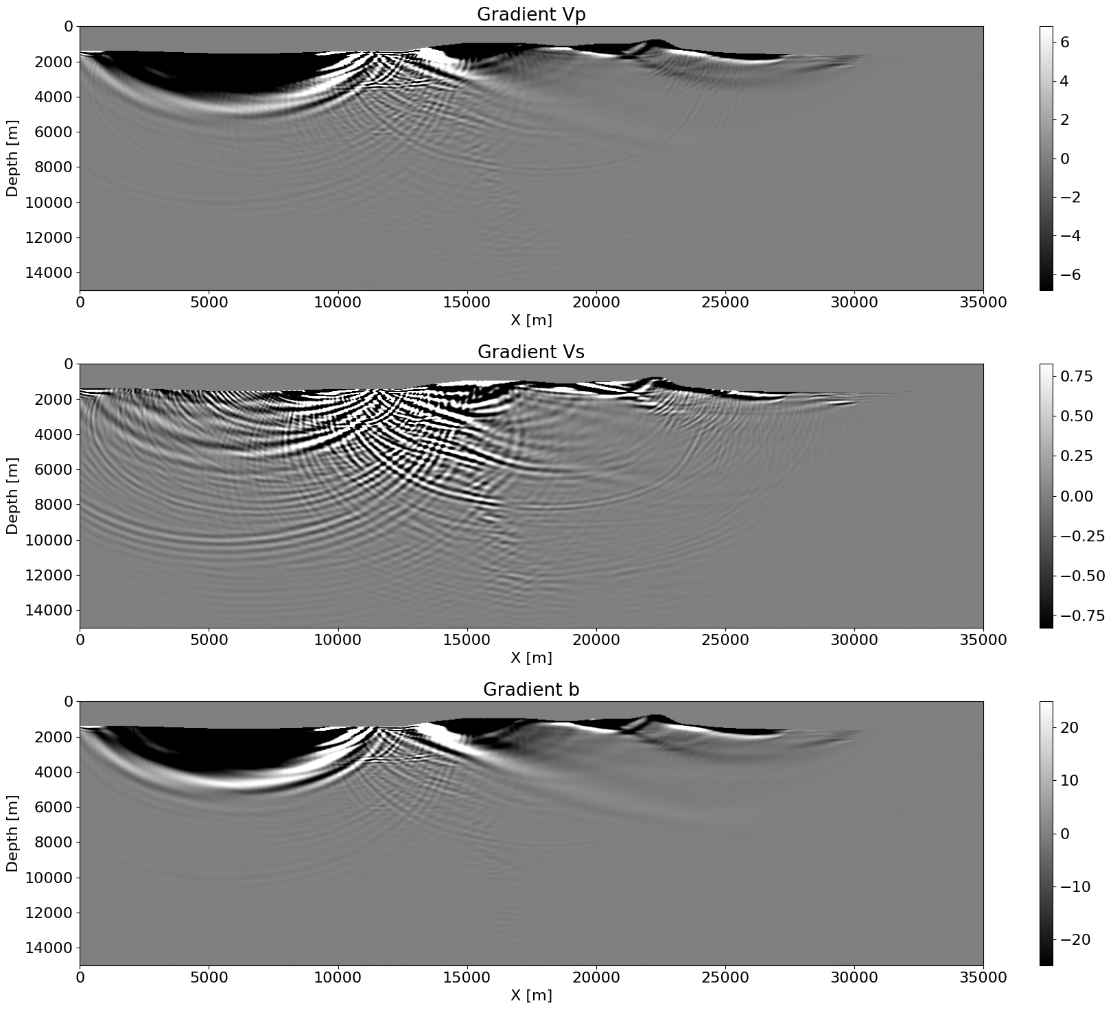
# Overlay gradient on the velocity model
plt.figure(figsize=(14, 10))

plt.subplot(2, 1, 1)
plot_simage(grad_vp.T, spacing=spacing,
            name='Vp gradient overlaid on true model',
            new_fig=False)
plot_velocity(vp_sub.T, spacing=spacing,
              alpha=0.4, new_fig=False)

plt.subplot(2, 1, 2)
plot_simage(grad_vs.T, spacing=spacing,
            name='Vs gradient overlaid on true model',
            new_fig=False)
plot_velocity(vs_sub.T, spacing=spacing,
              alpha=0.4, new_fig=False)

plt.tight_layout()
plt.show()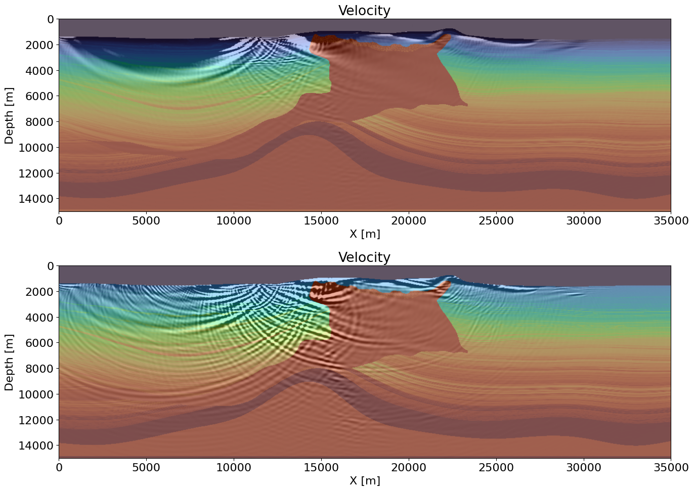
Summary
This tutorial demonstrated the complete workflow for elastic wave modeling and gradient computation with real-world data:
- Data I/O: Downloaded and read the SEAM 2D elastic model from SEG-Y files using
pysegy - Model setup: Built a
WaveModelfrom Vp, Vs, and density arrays with proper unit conversion (m/s to km/s, density to buoyancy) - Forward simulation: Ran the
iso-elasticsolver to generate a synthetic shot record - Gradient computation: Used the adjoint-state method to compute sensitivities with respect to Vp, Vs, and buoyancy
The gradient images highlight the model features that the data is most sensitive to, which is the starting point for full-waveform inversion (FWI).