import numpy as np
import matplotlib.pyplot as plt
from devito import Function
from recipes import layered_model, recipes_registryLinearized (Born) Modeling
This notebook demonstrates linearized forward modeling (Born modeling) in devitorecipes. Born modeling computes the scattered wavefield from a model perturbation — the action of the Jacobian \(J\) on a perturbation \(\delta m\):
\[\delta d = J \, \delta m\]
The operator couples two PDEs in a single run: 1. Background forward: propagates \(u\) with the physical source 2. Scattered field: propagates \(\delta u\) driven by the Born source \(\frac{\partial A}{\partial m} \delta m \, u\)
The scattered data \(\delta d\) is recorded at receivers.
Model setup
We create a layered acoustic true model, then derive a smooth background model from it. The velocity perturbation (reflectivity) is the difference between the two.
so = 8
nt = 2000
dt = .75

# True model (sharp layered interfaces)
model_true = layered_model('iso-acoustic', nlayers=3, shape=(301, 151),
                           spacing=(10., 10.), density=False, nbl=40,
                           space_order=so, fs=False, dt=dt)

# Smooth background model
model = layered_model('iso-acoustic', nlayers=3, shape=(301, 151),
                      spacing=(10., 10.), density=False, nbl=40,
                      space_order=so, fs=False, dt=dt)
model.smooth(['vp'], sigma=5)

extent = (model.grid.origin[0],
          model.grid.origin[0] + model.grid.extent[0],
          model.grid.origin[1] + model.grid.extent[1],
model.grid.origin[1])plt.figure(figsize=(14, 4))
plt.subplot(121)
plt.imshow(model_true.vp.data.T, cmap="jet", aspect="auto", extent=extent)
plt.colorbar(label="km/s")
plt.title("True P-wave velocity")
plt.xlabel("x [m]")
plt.ylabel("Depth [m]")
plt.subplot(122)
plt.imshow(model.vp.data.T, cmap="jet", aspect="auto", extent=extent)
plt.colorbar(label="km/s")
plt.title("Smooth background")
plt.xlabel("x [m]")
plt.ylabel("Depth [m]")
plt.tight_layout()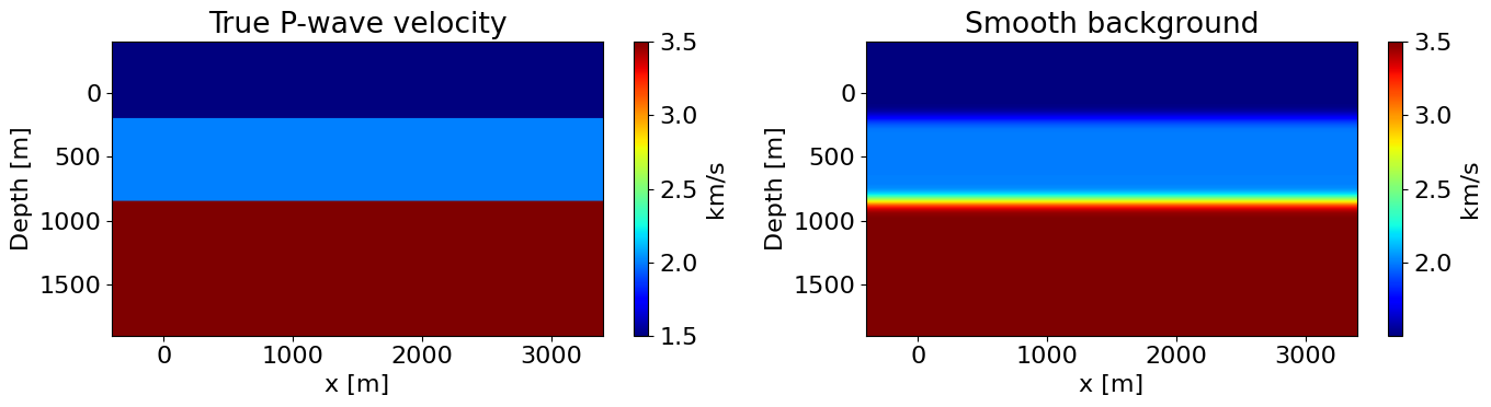
# Solver uses the smooth background model
solver = recipes_registry['iso-acoustic'](
    model, {'nt': nt, 'space_order': so, 'abox': False,
            'save': None, 't_sub': 1, 'f0': 0.015,
            'time_slots': 3, 'factorization': 0})
Model perturbation
The Born source reads a perturbation Function at runtime. We create a Function named dvp (matching the symbolic name used by born_source) and pass it to jacobian() as a keyword argument. This keeps the internal solver.perturbation('vp') clean for gradient accumulation.
# Reflectivity as a separate Function (not solver.perturbation)
dm = Function(name='dvp', grid=model.grid, space_order=solver.field_so)

# Only set perturbation inside the physical domain (not the absorbing boundary)
nbl = model.nbl
slc = tuple(slice(nbl, -nbl) for _ in dm.shape)
dm.data[slc] = (model_true.vp.data[slc] - model.vp.data[slc])plt.figure(figsize=(10, 4))
plt.imshow(dm.data.T, cmap="seismic", aspect="auto", extent=extent)
plt.colorbar(label="km/s")
plt.title("Velocity perturbation $\\delta v_p = v_{true} - v_0$")
plt.xlabel("x [m]")
plt.ylabel("Depth [m]")
plt.tight_layout()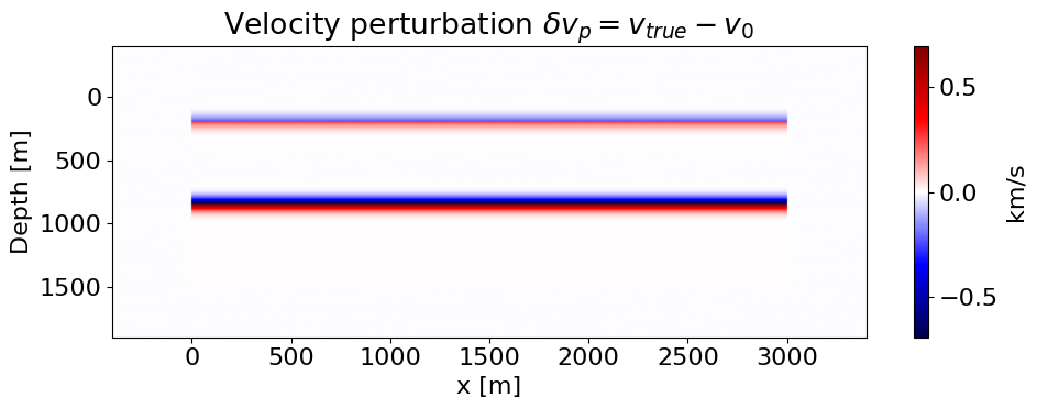
Born forward modeling
solver.jacobian(params='vp') runs both the background forward and the scattered field PDE in a single operator. The scattered data is recorded at receivers.
# Pass dvp=dm to override the symbolic perturbation at runtime
solver.rec.data.fill(0)
solver.jacobian(params='vp', dvp=dm)
born_data = solver.rec.data.copy()
Operator `dampvp` ran in 0.01 s
Operator `initdamp` ran in 0.01 s
Operator `JacobianAcousticIsotropic` ran in 0.45 splt.figure(figsize=(10, 4))
plt.imshow(born_data, cmap='seismic', aspect='auto',
vmin=-.1*np.max(np.abs(born_data)),
vmax=.1*np.max(np.abs(born_data)),
extent=(0, 3000, nt*dt/1000, 0))
plt.colorbar()
plt.title("Born (linearized) data $\\delta d = J \\, \\delta m$")
plt.xlabel("Receiver position [m]")
plt.ylabel("Time [s]")
plt.tight_layout()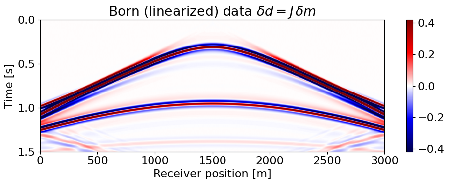
Comparison with nonlinear data difference
The Born data should approximate the difference between the true and background data for small perturbations.
# True data (nonlinear forward in true model)
solver.rec.data.fill(0)
solver.forward(vp=model_true.vp)
true_data = solver.rec.data.copy()

# Background data
solver.rec.data.fill(0)
solver.forward()
bg_data = solver.rec.data.copy()

# Nonlinear data difference
diff_data = true_data - bg_data
Operator `ForwardAcousticIsotropic` ran in 0.22 s
Operator `ForwardAcousticIsotropic` ran in 0.21 sclip = .1 * np.max(np.abs(diff_data))
plt.figure(figsize=(14, 4))
plt.subplot(131)
plt.imshow(diff_data, cmap='seismic', aspect='auto',
vmin=-clip, vmax=clip,
extent=(0, 3000, nt*dt/1000, 0))
plt.title("Nonlinear difference\n$F(m_{true}) - F(m_0)$")
plt.xlabel("Receiver position [m]")
plt.ylabel("Time [s]")
plt.subplot(132)
plt.imshow(born_data, cmap='seismic', aspect='auto',
vmin=-clip, vmax=clip,
extent=(0, 3000, nt*dt/1000, 0))
plt.title("Born data\n$J \\, \\delta m$")
plt.xlabel("Receiver position [m]")
plt.subplot(133)
plt.imshow(diff_data - born_data, cmap='seismic', aspect='auto',
vmin=-clip, vmax=clip,
extent=(0, 3000, nt*dt/1000, 0))
plt.title("Residual (nonlinear - Born)")
plt.xlabel("Receiver position [m]")
plt.tight_layout()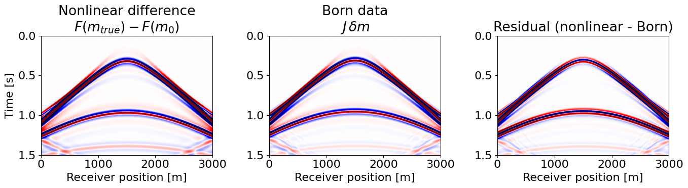
Taylor test
The Born data should match the linearization of the forward operator. We verify with the Taylor expansion:
\[\| F(m_0 + h \, \delta m) - F(m_0) \| = O(h)\] \[\| F(m_0 + h \, \delta m) - F(m_0) - h \, J \, \delta m \| = O(h^2)\]
from devito import initialize_function

vp0 = model.vp._rebuild(name='vp0')
vp_bg = model.vp.data.copy()
dp = dm.data.copy()

h0, rate = .5, 2.0
prev_e1, prev_e2 = 0.0, 0.0
for i in range(8):
    initialize_function(vp0, vp_bg + h0 * dp, 0)
    solver.rec.data.fill(0)
    solver.forward(vp=vp0)
    dF = solver.rec.data - bg_data
    e1 = np.linalg.norm(dF)
    e2 = np.linalg.norm(dF - h0 * born_data)
    r1 = prev_e1 / e1 if prev_e1 > 0 else 0
    r2 = prev_e2 / e2 if prev_e2 > 0 else 0
    print(f"h={h0:.3e}  |dF|={e1:.3e}  |dF-hJ|={e2:.3e}"
          f"  r1={r1:.2f}  r2={r2:.2f}")
    prev_e1, prev_e2 = e1, e2
    h0 /= rate

print(f"\nExpected: r1 ~ {rate:.1f}, r2 ~ {rate**2:.2f}")
Operator `ForwardAcousticIsotropic` ran in 0.24 sh=5.000e-01 |dF|=1.572e+02 |dF-hJ|=8.433e+01 r1=0.00 r2=0.00Operator `ForwardAcousticIsotropic` ran in 0.21 sh=2.500e-01 |dF|=7.460e+01 |dF-hJ|=2.006e+01 r1=2.11 r2=4.20Operator `ForwardAcousticIsotropic` ran in 0.23 sh=1.250e-01 |dF|=3.598e+01 |dF-hJ|=4.834e+00 r1=2.07 r2=4.15Operator `ForwardAcousticIsotropic` ran in 0.23 sh=6.250e-02 |dF|=1.763e+01 |dF-hJ|=1.185e+00 r1=2.04 r2=4.08Operator `ForwardAcousticIsotropic` ran in 0.21 sh=3.125e-02 |dF|=8.725e+00 |dF-hJ|=2.936e-01 r1=2.02 r2=4.03Operator `ForwardAcousticIsotropic` ran in 0.22 sh=1.562e-02 |dF|=4.351e+00 |dF-hJ|=8.118e-02 r1=2.01 r2=3.62Operator `ForwardAcousticIsotropic` ran in 0.21 sh=7.812e-03 |dF|=2.166e+00 |dF-hJ|=2.535e-02 r1=2.01 r2=3.20Operator `ForwardAcousticIsotropic` ran in 0.21 sh=3.906e-03 |dF|=1.085e+00 |dF-hJ|=1.195e-02 r1=2.00 r2=2.12
Expected: r1 ~ 2.0, r2 ~ 4.00Adjoint test (dot-product test)
The Born forward \(J\) and the gradient \(J^T\) must satisfy the adjoint relationship:
\[\langle J \, \delta m, \, d \rangle = \langle \delta m, \, J^T d \rangle\]
We verify this with random \(\delta m\) and \(d\). The ratio should be \(\approx 1\).
rng = np.random.RandomState(42)

# Random model perturbation
dm_rand = Function(name='dvp', grid=model.grid,
                   space_order=solver.field_so)
dm_data = np.zeros(dm_rand.shape, dtype=np.float32)
inner = tuple(slice(nbl + 10, -(nbl + 10)) for _ in dm_rand.shape)
dm_data[inner] = rng.randn(*dm_data[inner].shape).astype(
    np.float32) * 1e-3
dm_rand.data[:] = dm_data

# Born forward: dd = J * dm
solver.rec.data.fill(0)
solver.jacobian(params='vp', dvp=dm_rand)
born_rand = solver.rec.data.copy()

# Random data perturbation
d_rand = solver.rec.copy()
d_rand.data[:] = rng.randn(*d_rand.data.shape).astype(np.float32)

# Adjoint: g = J^T * d
solver.perturbation(param='vp').data.fill(0)
solver.forward(save=True)
solver.jacobian_adjoint(rec=d_rand, params='vp')
g_adj = solver.perturbation(param='vp').data.copy()

# Dot-product: <J dm, d> ~ <dm, J^T d>
lhs = dt * np.dot(born_rand.ravel(), d_rand.data.ravel())
rhs = np.dot(dm_data.ravel(), g_adj.ravel())
print(f"<J dm, d>   = {lhs:.6e}")
print(f"<dm, J^T d> = {rhs:.6e}")
print(f"Ratio       = {lhs / rhs:.6f}")
Operator `JacobianAcousticIsotropic` ran in 0.44 s
Operator `ForwardAcousticIsotropic` ran in 1.77 s
Operator `JacobianAdjAcousticIsotropic` ran in 1.12 s<J dm, d> = 4.745799e+00
<dm, J^T d> = 4.745677e+00
Ratio = 1.000026Gradient (migration image)
The adjoint Jacobian \(J^T\) maps data to model space. Applied to the data residual, it produces the FWI gradient — a migration image that locates the reflectors.
# Compute gradient from the data residual
residual = solver.rec.copy()
residual.data[:] = bg_data - true_data

# Zero the gradient accumulator before adjoint
solver.perturbation(param='vp').data.fill(0)
solver.forward(save=True)
solver.jacobian_adjoint(rec=residual, params='vp')
g = solver.perturbation(param='vp').data
Operator `ForwardAcousticIsotropic` ran in 0.51 s
Operator `JacobianAdjAcousticIsotropic` ran in 0.33 sclip_g = .5 * np.max(np.abs(g))
plt.figure(figsize=(14, 4))
plt.subplot(121)
plt.imshow(dm.data.T, cmap="seismic", aspect="auto", extent=extent)
plt.colorbar(label="km/s")
plt.title("True perturbation $\\delta m$")
plt.xlabel("x [m]")
plt.ylabel("Depth [m]")
plt.subplot(122)
plt.imshow(g.T, cmap="seismic", aspect="auto", extent=extent,
vmin=-clip_g/1000, vmax=clip_g/1000)
plt.colorbar()
plt.title("Gradient (migration image) $J^T \\delta d$")
plt.xlabel("x [m]")
plt.ylabel("Depth [m]")
plt.tight_layout()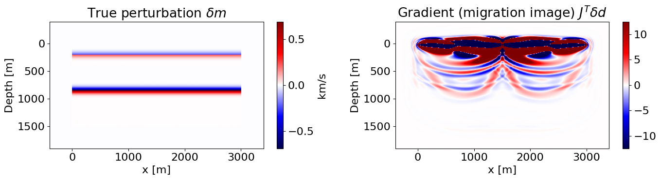
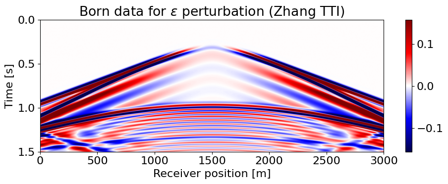
TTI Born modeling
The same interface works for anisotropic (TTI) models. The Born source for Thomsen parameters uses direct operator derivatives (no PDE identity needed).
model_tti = layered_model('tti-zhang', nlayers=3, shape=(301, 151),
                         spacing=(10., 10.), density=False, nbl=40,
                         space_order=so, fs=False, dt=dt)

solver_tti = recipes_registry['tti-zhang'](
    model_tti, {'nt': nt, 'space_order': so, 'abox': False,
                'save': None, 't_sub': 1, 'f0': 0.015,
                'time_slots': 3, 'factorization': 0})

# Epsilon perturbation as a separate Function
deps = Function(name='depsilon', grid=model_tti.grid,
                space_order=solver_tti.field_so)
deps.data[:] = 0.05 * (model_tti.eps.data[:] > 0)

solver_tti.rec.data.fill(0)
solver_tti.jacobian(params='epsilon', depsilon=deps)
born_eps = solver_tti.rec.data.copy()
Operator `dampvp` ran in 0.01 s
Operator `initdamp` ran in 0.01 s
Operator `JacobianZhangTTI` ran in 1.41 splt.figure(figsize=(10, 4))
clip = .1 * np.max(np.abs(born_eps))
plt.imshow(born_eps, cmap='seismic', aspect='auto',
vmin=-clip, vmax=clip,
extent=(0, 3000, nt*dt/1000, 0))
plt.colorbar()
plt.title("Born data for $\\epsilon$ perturbation (Zhang TTI)")
plt.xlabel("Receiver position [m]")
plt.ylabel("Time [s]")
plt.tight_layout()