import os
os.environ['OMP_NUM_THREADS'] = '8'
os.environ['DEVITO_LOGGING'] = 'WARNING'

import matplotlib.pyplot as plt
import numpy as np

from recipes import recipes_registry, layered_modelImaging conditions
A migration or a gradient is a correlation of two wavefields: the source wavefield \(u\), propagated forward, and the receiver wavefield \(\bar u\), propagated backward from the data residual. How they are correlated is the imaging condition, and the choice decides what ends up in the image — a reflectivity, a velocity update, or a superposition of the two that is useful for neither.
Recipes accumulate three of them. They are selected by the parameter you ask jacobian_adjoint for, because each one is the gradient with respect to a different parameter — there is no separate switch:
params= |
kernel | this is |
|---|---|---|
'm' |
\(u_{tt}\,\bar u\) | the plain cross-correlation, the squared-slowness gradient |
'Z' |
\(m\,u\,\bar u_{tt} + \nabla u\cdot\nabla\bar u\) | the inverse-scattering condition, the impedance gradient |
'mZ' |
\(m\,u\,\bar u_{tt} - \nabla u\cdot\nabla\bar u\) | its complement, the slowness-at-fixed-impedance gradient |
Elsewhere these go by other names. Z is JUDI’s ic="isic" and mZ is its ic="fwi"; the literature calls the pair the inverse-scattering imaging condition and its transmission complement. The signs and the \(m\) weight are the same in both codes.
The reason the recipes name them after parameters rather than after imaging conditions is that they are gradients, and are verified as such: every one of them passes a Taylor test and a directional-derivative check on all three recipes that implement them (docs/gradients.qmd).
Setup
One source and one receiver, so the kernels are the textbook pictures rather than a stack of them.
time_slots=3 is required. Both conditions take a second time derivative of the adjoint field, and two buffers alias \(t+1\) onto \(t-1\) — the mass kernel then comes back wrong by enough to swamp the stiffness one, with Z and mZ landing 99.96 per cent correlated instead of essentially uncorrelated. Asking for either with time_slots=2 raises rather than doing that quietly.
so, dt, nt, f0 = 8, 0.75, 2600, 0.008
CONDITIONS = ('m', 'Z', 'mZ')


def build(nlayers, homogeneous=False):
    model = layered_model('iso-acoustic', nlayers=nlayers, shape=(181, 181),
                          spacing=(10., 10.), density=True, nbl=40,
                          space_order=so, dt=dt, smooth=False)
    if homogeneous:
        model.vp.data[:] = float(np.array(model.vp.data).min())
        model.b.data[:] = float(np.array(model.b.data).max())

    solver = recipes_registry['iso-acoustic'](
        model, {'nt': nt, 'space_order': so, 'f0': f0,
                't_sub': 1, 'time_slots': 3, 'factorization': 0,
                'abox': False, 'save': None})
    return model, solver
A pure transmission experiment
Put the source at depth and keep one surface trace. In a homogeneous model the only event in that trace is the transmitted wave, so whatever the kernel looks like is the transmission kernel — the low-wavenumber “banana” that swamps a reflectivity image, and the signal a velocity update lives on.
model, solver = build(1, homogeneous=True)

extent = np.array(model.domain_size, dtype=np.float32)
solver.src.coordinates.data[0, 0] = extent[0] / 2
solver.src.coordinates.data[0, -1] = 0.7 * extent[-1]

solver.forward(save=True)

trace = int(0.78 * solver.rec.data.shape[1])
residual = solver.rec.copy()
keep = residual.data[:, trace].copy()
residual.data[:] = 0
residual.data[:, trace] = keep

src_xz = solver.src.coordinates.data[0].copy()
rec_xz = solver.rec.coordinates.data[trace].copy()
print('source', src_xz, 'receiver', rec_xz)
source [ 900. 1260.] receiver [1400. 12.5]solver.rec.copy() returns the receiver itself, not a copy. Do not run a forward between building residual and correlating it: it refills the record and undoes the mute and the trace selection above, silently, and the image still looks like an image.
One forward is enough for all three conditions — the saved wavefield survives an adjoint pass, and a second jacobian_adjoint with no fresh forward reproduces the same kernel to 6e-7. What does not reset is the accumulator: jacobian_adjoint increments the field perturbation returns rather than overwriting it (that is how a shot loop sums), so re-running for the same parameter doubles it.
def correlate(solver, residual):
    images = {}
    for param in CONDITIONS:
        solver.perturbation(param=param).data[:] = 0
        solver.jacobian_adjoint(rec=residual, params=param)
        images[param] = np.array(solver.perturbation(param=param).data)
    return images


transmission = correlate(solver, residual)
TITLES = {'m': 'm — cross-correlation\n$u_{tt}\\,\\bar u$',
'Z': 'Z — impedance (ISIC)\n$m\\,u\\,\\bar u_{tt} + '
'\\nabla u\\cdot\\nabla\\bar u$',
'mZ': 'mZ — slowness at fixed Z\n$m\\,u\\,\\bar u_{tt} - '
'\\nabla u\\cdot\\nabla\\bar u$'}
def far_field(model, coords, shape, radius=300.):
"""Away from the source and the receiver, where every kernel is
singular and none of them cancels."""
nbl = model.nbl
inner = tuple(np.array(shape) - 2 * nbl)
spacing = np.array(model.spacing, dtype=np.float32)
xx = np.arange(inner[0])[:, None] * spacing[0]
zz = np.arange(inner[1])[None, :] * spacing[1]
far = np.ones(inner, dtype=bool)
for pt in coords:
far &= ((xx - pt[0]) ** 2 + (zz - pt[-1]) ** 2) > radius ** 2
return far
def show(images, model, coords, suptitle):
nbl = model.nbl
far = far_field(model, coords, images['m'].shape)
# Scale off the far field: a max-normalized image is blank everywhere
# except the two singular points.
scale = max(np.percentile(np.abs(g[nbl:-nbl, nbl:-nbl][far]), 99.5)
for g in images.values())
ex = np.array(model.domain_size) / 1e3
fig, axes = plt.subplots(1, 3, figsize=(15, 4.6))
for ax, param in zip(axes, CONDITIONS):
ax.imshow(images[param][nbl:-nbl, nbl:-nbl].T, cmap='seismic',
vmin=-scale, vmax=scale, aspect='auto',
extent=(0, ex[0], ex[-1], 0), interpolation='bilinear')
for pt, marker in zip(coords, ('*', 'v')):
ax.plot(pt[0] / 1e3, pt[-1] / 1e3, marker, color='black', ms=12,
mec='white', mew=1., clip_on=False)
ax.set_title(TITLES[param])
ax.set_xlabel('x (km)')
axes[0].set_ylabel('depth (km)')
fig.suptitle(suptitle)
fig.tight_layout()
show(transmission, model, (src_xz, rec_xz),
'homogeneous — the only event is the transmitted wave '
'(star: source, triangle: receiver)')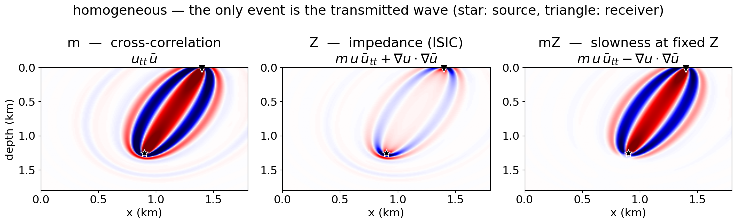
m is the whole banana. Z has cancelled it. mZ has kept it.
The cancellation is a scattering-angle argument. Write both fields locally as plane waves, \(u\sim e^{i(k_u\cdot x-\omega t)}\) and \(\bar u\sim e^{i(k_{\bar u}\cdot x-\omega t)}\). Then \(m\,u\,\bar u_{tt}\) is \(-|k|^2u\bar u\) regardless of direction, while \(\nabla u\cdot\nabla\bar u\) is \(-(k_u\cdot k_{\bar u})u\bar u\). The two are equal when the wavefields are parallel and equal-and-opposite when they are anti-parallel, so the sum and the difference each annihilate one of the two cases.
Measured away from the two singular points, where nothing cancels:
nbl = model.nbl
far = far_field(model, (src_xz, rec_xz), transmission['m'].shape)


def rms(image):
    return float(np.sqrt((image[nbl:-nbl, nbl:-nbl][far] ** 2).mean()))


reference = rms(transmission['m'])
for param in CONDITIONS:
    print(f'{param:>3s}  {rms(transmission[param]) / reference:.3f}'
          f'  of the cross-correlation kernel')
m 1.000 of the cross-correlation kernel
Z 0.079 of the cross-correlation kernel
mZ 0.828 of the cross-correlation kernelZ keeps about a tenth of it and mZ about four fifths. That is the assertion in test_isic_suppresses_transmission.
A reflection
Now a two-layer model, with source and receiver both at the surface, and the direct arrival muted out of the residual. What is left in the trace is the reflection.
model2, solver2 = build(2)

extent = np.array(model2.domain_size, dtype=np.float32)
solver2.src.coordinates.data[0, 0] = extent[0] / 3
solver2.src.coordinates.data[0, -1] = 1.25 * model2.spacing[-1]

solver2.forward(save=True)

trace2 = int(0.62 * solver2.rec.data.shape[1])
residual2 = solver2.rec.copy()
keep2 = residual2.data[:, trace2].copy()
residual2.data[:] = 0
residual2.data[:, trace2] = keep2

# Mute out to the direct arrival plus a wavelet length, with a short taper.
src_x = float(solver2.src.coordinates.data[0, 0])
rec_x = float(solver2.rec.coordinates.data[trace2, 0])
t_direct = abs(rec_x - src_x) / float(np.array(model2.vp.data).max()) + 1.5 / f0
cut = min(int(t_direct / model2.critical_dt), residual2.data.shape[0])
taper = int(0.5 / f0 / model2.critical_dt)
residual2.data[:cut, trace2] = 0
end = min(cut + taper, residual2.data.shape[0])
residual2.data[cut:end, trace2] *= np.linspace(0, 1, end - cut)

reflection = correlate(solver2, residual2)
show(reflection, model2,
     (solver2.src.coordinates.data[0].copy(),
      solver2.rec.coordinates.data[trace2].copy()),
     'two layers — direct arrival muted, so the event is the reflection')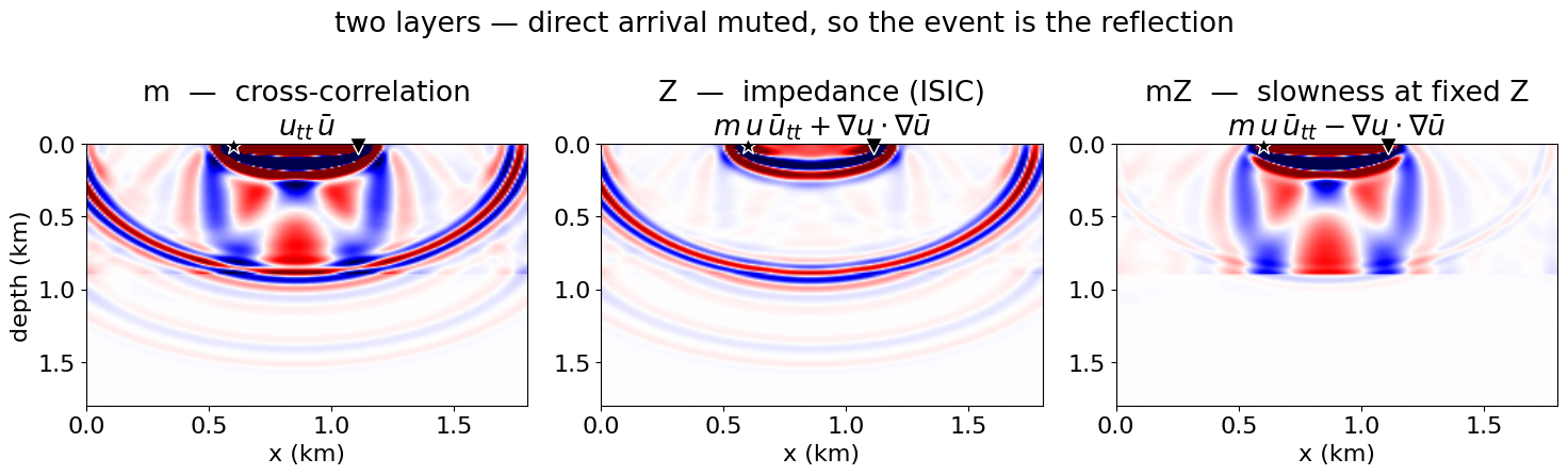
The reflector sits at about 0.85 km.
mimages it, and also carries the transmission “rabbit ears” between source and receiver — an artifact that in a real image is stronger than the reflector and is usually attacked afterwards with a Laplacian or a taper.Zimages the reflector and has removed the rabbit ears. No filter applied.mZhas cancelled the reflector and kept only the rabbit ears.
Choosing
- RTM / LSRTM —
Z. The transmission artifact is the thing that ruins a reflectivity image, and this is the condition that removes it at the source rather than afterwards. - Conventional FWI —
m. The update is meant to be dominated by the transmitted wave, so there is nothing to cancel, and the plain cross-correlation is the gradient of the objective being minimized. - Reflection FWI — both. The reflectivity is inverted on
Zat a fixed background and the background is updated onmZ, which sees only the long wavelengths.mZis squared slowness at fixed impedance, so moving along it changes the kinematics without perturbing the reflectors: \(\delta\ln c = -\tfrac12\delta\ln m\) with \(\delta\ln\rho = +\tfrac12\delta\ln m\) leaves \(Z=\rho c\) alone.
Notes
Cost. Both conditions read the saved forward wavefield the way m does and add a gradient correlation on top of the mass one — a handful of first derivatives per time step. Memory is unchanged: Z and mZ accumulate into a single field like any other parameter.
Discretization. The stiffness term is taken on the half cells, where b is sampled, and not at the node. That is not an aesthetic choice: the node-centred \(\nabla u\cdot\nabla\bar u\) is the right expression in the continuum but not the derivative of the discrete objective, and using it puts the Z gradient 9 per cent off a finite difference and makes the error drift with the model size.
Anisotropy. Z and mZ are implemented for iso-acoustic, tti-zhang and tti-fletcher. The anisotropic recipes carry the Thomsen weights through both kernels — the two equations cross-couple, so the stiffness term pairs each field with both adjoint fields — and reduce to the isotropic condition when the anisotropy is zeroed. Zhang matches the isotropic image bit for bit; Fletcher matches it once both are smoothed over two cells, because it writes the Laplacian expanded rather than in conservative form and the transpose of that onto b is an 8-point stencil that rings at the grid scale. The gradient is unaffected (Fletcher’s Z matches a central difference at 0.9994); the image is not smooth.
The elastic recipes do not implement them: the condition above is written for a scalar wave equation with one stiffness, and the elastic analogue needs the full \(C_{ijkl}\) contraction rather than a two-term correlation.